数据结构与算法(java版)

文章目录
[TOC]
引子
数据结构包括:线性结构和非线性结构
- 线性结构
- 特点:数据元素一对一的线性关系
- 线性结构有两种不同的存储结构:一种是顺序存储结构,元素处于相邻地址空间,顺序存储的线性表又称为顺序表;另一种是链式存储结构,元素节点保存数据元素和相邻元素地址信息,相邻元素不一定在地址空间上连续。
- 常见的线性结构:数组、队列、链表和栈
- 非线性结构
- 常见的有:二维数组、多维数组、广义表、树结构、图结构
时间复杂度
-
时间频度:一个算法花费的时间与算法中语句的执行次数成正比例,哪个算法中语句执行次数多,它花费时间就多。**一个算法中的语句执行次数成为语句频度或时间频度。**记为
T(n)(注意:是语句重复执行的次数,而不是语句条数) -
时间复杂度:一般情况下,算法的基本操作语句的重复执行次数是问题规模n的某个函数,用
T(n)表示,若有某个辅助函数f(n),使得当n趋于无穷大时,T(n)/f(n)的极限值为不等于零的常熟,则成f(n)是T(n)的同数量级函数,记作**T(n)=O{f(n)},称O{f(n)}为算法的渐进时间复杂度,简称时间复杂度**。时间频度不同,但时间复杂度可能相同。
举例说明
T(n)=n²+7n+6与T(n)=3n²+2n+2它们的T(n)不同,但时间复杂度相同,都为O(n²) -
计算时间复杂度的方法
- 用常数1代替运行时间中的所有加法常数
T(n) = n²+7n+6=>T(n) = n²+7n+1 - 修改后的运行次数函数中,只保留最高阶项
T(n) = n²+7n+1=>T(n) = n² - 去除最高阶项的系数
T(n) = n²=>T(n) = n²=>O(n²)
- 用常数1代替运行时间中的所有加法常数
-
常见的时间复杂度
-
常数阶
O(1)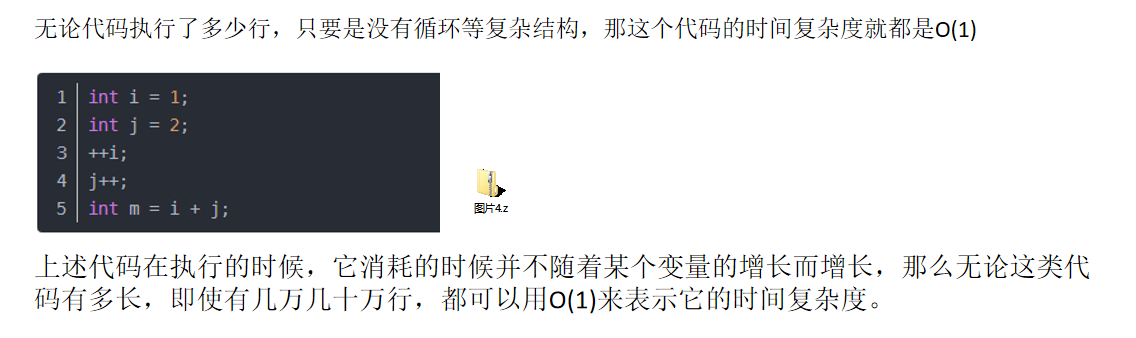
-
对数阶
O(log2n):以2为底,n为对数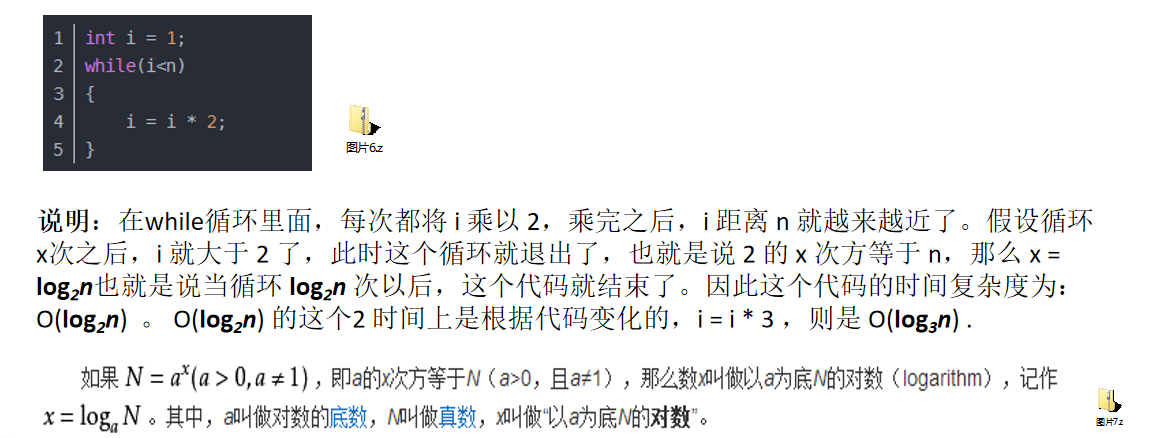
-
线性阶
O(n)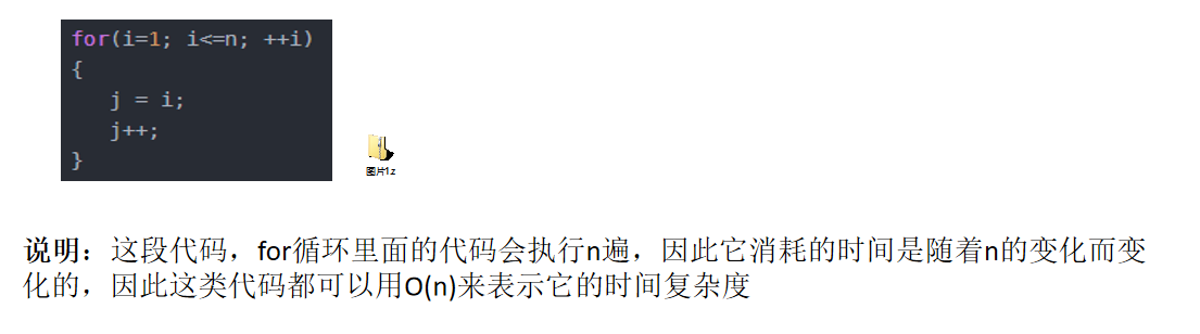
-
线性对数阶
O(nlog2n)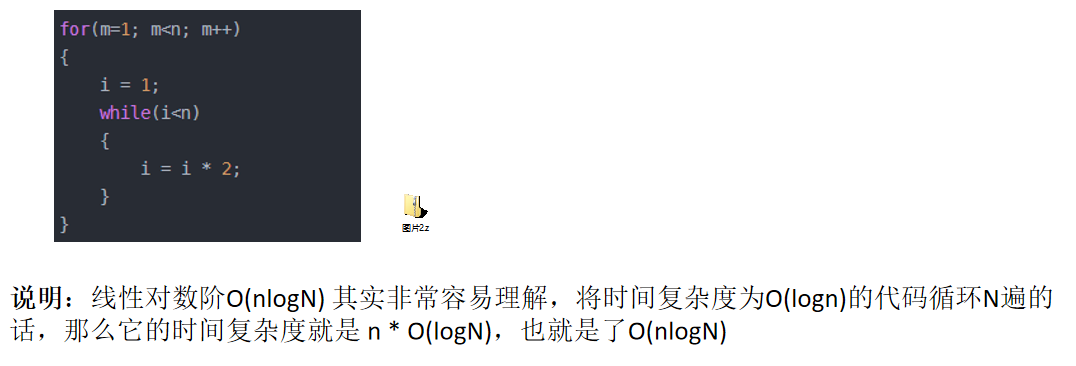
-
平方阶
O(n^2)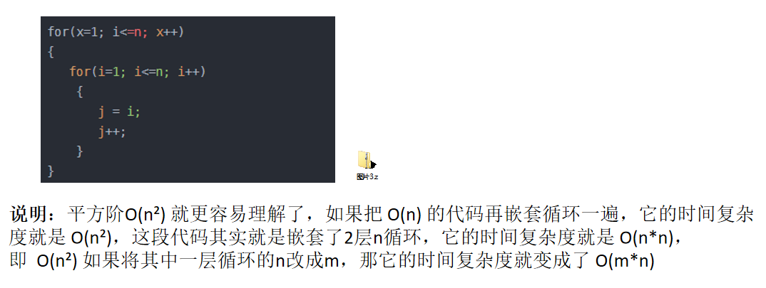
-
立方阶
O(n^3)参考上面的
O(n²)去理解就好了,O(n³)相当于三层n循环,其它的类似 -
k次方阶
O(n^k)参考上面的
O(n²)去理解就好了,O(n³)相当于三层n循环,其它的类似 -
指数阶
O(2^n)我们应该尽可能避免使用指数阶的算法常见的算法时间复杂度由小到大依次为:Ο(1)<Ο(log2n)<Ο(n)<Ο(nlog2n)<Ο(n2)<Ο(n3)< Ο(nk) <Ο(2n) ,随着问题规模n的不断增大,上述时间复杂度不断增大,算法的执行效率越低
-
-
平均时间复杂度和最坏时间复杂度
-
平均时间复杂度是指所有可能的输入实例均以等概率出现的情况下,该算法的运行时间。
-
最坏情况下的时间复杂度称最坏时间复杂度。一般讨论的时间复杂度均是最坏情况下的时间复杂度。 这样做的原因是:最坏情况下的时间复杂度是算法在任何输入实例上运行时间的界限,这就保证了算法的运行时间不会比最坏情况更长。
-
平均时间复杂度和最坏时间复杂度是否一致,和算法有关。
-
空间复杂度
- 类似于时间复杂度的讨论,一个算法的空间复杂度(
Space Complexity)定义为该算法所耗费的存储空间,它也是问题规模n的函数。 - 空间复杂度(Space Complexity)是对一个算法在运行过程中临时占用存储空间大小的量度。有的算法需要占用的临时工作单元数与解决问题的规模n有关,它随着n的增大而增大,当n较大时,将占用较多的存储单元,例如快速排序和归并排序算法就属于这种情况
- 在做算法分析时,主要讨论的是时间复杂度。从用户使用体验上看,更看重的程序执行的速度。一些缓存产品(
redis,memcache)和算法(基数排序)本质就是用空间换时间.
一、稀疏数组
-
原理
原始数组之中有很多重复或无用的数据,可以通过记录大量重复数据的位置和值来代替原来的重复数据,从而达到压缩的目的。
-
处理方法
- 记录数组一共几行几列,有多少个不同的值
- 把具有不同数值的元素行列记录至一个新的数组中(这个数组肯定会小于原先的数组),从而达到压缩的目的。
-
代码
 1
 2
 3
 4
 5
 6
 7
 8
 9
10
11
12
13
14
15
16
17
18
19
20
21
22
23
24
25
26
27
28
29
30
31
32
33
34
35
36
37
38
39
40
41
42
43
44
45
46
47
48
49
50
51
52
53
54
import java.util.Arrays; public class first { public static void main(String[] args) { //初始化二维数组 int[][] oldArray =new int[10][10]; oldArray[1][3]=1; oldArray[2][7]=3; oldArray[5][2]=10; System.out.println(Arrays.deepToString(oldArray)); int validNum =0; //获取不同值个数 for (int i=0;i<oldArray.length;i++){ for (int j=0;j<oldArray[i].length;j++){ //将非重复元素存到压缩数组 if (oldArray[i][j]!=0){ validNum++; } } } //初始化稀疏数组,确定深度 int[][] parseArray =new int[validNum+1][3]; int index=0; //初始化稀疏数组第一个索引,用来表示原数组的个数及值重值 parseArray[0][0]=oldArray.length; parseArray[0][1]=oldArray[0].length; parseArray[0][2]=0; for (int i=0;i<oldArray.length;i++){ for (int j=0;j<oldArray[i].length;j++){ //将非重复元素存到压缩数组 if (oldArray[i][j]!=0){ index++; //记录非零值 parseArray[index][0]=i; parseArray[index][1]=j; parseArray[index][2]=oldArray[i][j]; } } } //稀疏数组结果 System.out.println(Arrays.deepToString(parseArray)); //还原稀疏数组 //初始化稀疏数组大小 int[][] newArray =new int[parseArray[0][0]][parseArray[0][1]]; //读取稀疏数组数值 for (int i=1;i<parseArray.length;i++){ newArray[parseArray[i][0]][parseArray[i][1]]=parseArray[i][2]; } System.out.println(Arrays.deepToString(newArray)); } }
二、队列
1. 非循环队列(一般不使用)
-
原理
-
队列是一个有序列表,可以使用数组或者链表实现。数组的特点是相邻地址索引快,读操作效率更高;链表是链式存储,写操作效率更高
-
遵循先入先出的原则
-
示意图
-
-
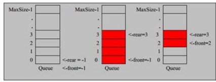
处理方法(数组)
-
队列初始化时,默认
front==rear==-1,头指针始终指向队列第一个元素的前一个索引位置(不一定存在),;尾指针始终指向队列队后一个元素的索引位置 -
队列元素增加:尾指针后移,
rear+1,当rear=maxSize-1表示队列已满 -
队列元素取出:头指针后移,
front-1,当front==rear表示队列已空
-
-
代码实现
 1
 2
 3
 4
 5
 6
 7
 8
 9
10
11
12
13
14
15
16
17
18
19
20
21
22
23
24
25
26
27
28
29
30
31
32
33
34
35
36
37
38
39
40
41
42
43
44
45
46
47
48
49
50
public class queue { //队列深度 private int maxSize; //队头指针 private int front; //队尾指针 private int rear; //队列元素使用数组作为队列结构 private int[] arr; //添加队列元素 public void addQueue(int e){ if (isFull()){ System.out.println("the queue is full..."); return; } this.rear++; this.arr[this.rear]=e; } //取出队列元素 public int getQueue(){ //判断队列是否为空 if (isEmpty()){ throw new RuntimeException("the queue is empty..."); } this.front++; return this.arr[this.front]; } //显示队列数据 public void list() { for (int v : arr) { System.out.print(v+" "); } } //判断队列是否已满 public boolean isFull(){ return this.maxSize-1==this.rear; } //判断队列是否为空 public boolean isEmpty(){ return this.rear==this.front; } //构造队列 public queue(int maxSize) { this.maxSize = maxSize; this.front = -1; this.rear = -1; this.arr = new int[maxSize]; } }
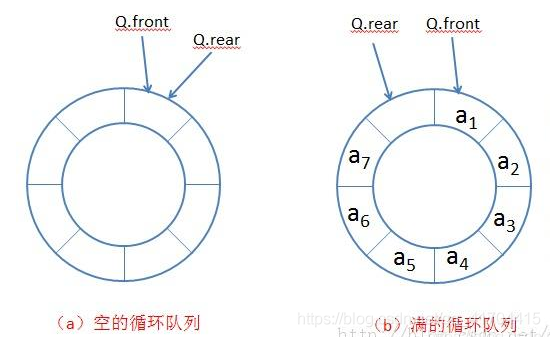
2. 循环队列
-
非循环队列的缺陷
非循环队列的空间不能反复利用,队列空间一旦填满不能再对队列进行写操作。其问题在于,非循环队列元素添加的实现只是简单的将队列进行后移,每添加一次元素,
rear后移一个位置,直到rear==maxSize-1时,不能再往后移(队列已满)。也就是说,目前数组使用一次就不能使用了,比较浪费但是可以通过对队列的指针取余(也叫取模),可以解决这个缺陷。内存上并没有环形的结构,因此环形队列实际上是数组的线性空间来实现的。当数据到了尾部应该怎么处理呢?它将转回到原来位置进行处理,通过取模操作来实现
所谓取模,只是将不断增大的
rear通过取模(取余)的方式,将rear大小不断缩小在一个“环”里,rear沿着“环”走 -
原理图
-
处理方法
front头指针指向队列第一个元素;rear尾指针指向队列最后一个元素的后一个位置。(与非循环队列相反)- 队满时,
(rear+1)%maxSize==front,意即rear后一个位置的下一个元素如果是front,表示队列已满 - 队空时,
rear==front - 队列初始化时,
rear==front==0 - 队列之中的有效数据个数:
(rear+maxSize-front)%maxSize或者Math.abs(rear-front),两者结果一样,因为rear与front的差值不可能查过maxSize
-
代码实现
 1
 2
 3
 4
 5
 6
 7
 8
 9
10
11
12
13
14
15
16
17
18
19
20
21
22
23
24
25
26
27
28
29
30
31
32
33
34
35
36
37
38
39
40
41
42
43
44
45
public class circleQueue { private int maxSize; private int front; private int rear; private int[] arr; //判断队列是否为空 public boolean isEmpty(){ return this.front==this.rear; } //判断队列是否满了 public boolean isFull(){ return (this.rear+1)%maxSize==this.front; } //添加队列元素 public void addQueue(int e){ if (isFull()){ throw new RuntimeException("queue is full\n"); } this.arr[this.rear]=e; //注意取模 this.rear=(this.rear+1)%this.maxSize; } //取出队列元素 public int getQueue(){ if (isEmpty()){ throw new RuntimeException("queue is empty\n"); } int v = arr[front]; //取模 front=(front+1)%maxSize; return v; } //获取有效个数 public void list(){ for (int i = 0; i < (rear + maxSize - front) % maxSize; i++) { System.out.print(arr[front+i]+" "); } } public circleQueue(int maxSize) { this.maxSize = maxSize; this.front=0; this.rear=0; this.arr=new int[maxSize]; } }
三、链表
1. 单链表
-
原理
-
链表是以节点的方式存储的,每个节点包含data域(存放数据)、next域(指向下一个节点)
-
链表的各个节点地址不一定是连续
-
链表分类:带头节点的链表和没有头节点的链表。
-
原理图
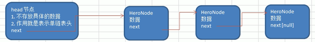
head头节点:不存放数据
-
-
处理方法
- 创建一个head头节点。作用是表示整个链表的地址
- 添加一个节点就将链表的最后一个节点的next域指向这个节点
- 插入一个节点就先遍历链表找出需要插入的位置,然后让指针插入对应即可
- 删除一个节点就先遍历找到这个节点,然后将这个节点的前后节点指针相连,这个节点就没有指针指向他,在
java中会被垃圾回收机制回收
-
代码实现
  1
  2
  3
  4
  5
  6
  7
  8
  9
 10
 11
 12
 13
 14
 15
 16
 17
 18
 19
 20
 21
 22
 23
 24
 25
 26
 27
 28
 29
 30
 31
 32
 33
 34
 35
 36
 37
 38
 39
 40
 41
 42
 43
 44
 45
 46
 47
 48
 49
 50
 51
 52
 53
 54
 55
 56
 57
 58
 59
 60
 61
 62
 63
 64
 65
 66
 67
 68
 69
 70
 71
 72
 73
 74
 75
 76
 77
 78
 79
 80
 81
 82
 83
 84
 85
 86
 87
 88
 89
 90
 91
 92
 93
 94
 95
 96
 97
 98
 99
100
101
102
103
104
105
106
107
108
109
110
111
112
113
114
115
116
117
118
119
120
121
122
123
124
125
126
127
128
129
130
131
132
133
134
135
136
137
138
139
140
141
142
143
144
145
public class singleLinkedList { public static void main(String[] args) { heroNode h1 = new heroNode(1, "刘海斌"); heroNode h2 = new heroNode(2, "包文杰"); heroNode h3 = new heroNode(3, "王铁霖"); heroNode h4 = new heroNode(4, "牟国柱"); managerSingleList manager = new managerSingleList(); manager.addNode(h1); manager.addNode(h2); manager.addNode(h3); manager.addNode(h4); manager.showList(); manager.updateList("cold bin", 1); manager.insertNode(new heroNode(0, "无"), 1); manager.showList(); manager.delNode(3); manager.showList(); } } class managerSingleList { //头节点 private heroNode head; public managerSingleList() { this.head = new heroNode(0, ""); } //添加 public void addNode(heroNode node) { //遍历链表至最后一个节点 heroNode temp = head; while (temp.next != null) { temp = temp.next; } //插入尾节点 temp.next = node; node.next = null; System.out.println("添加成功"); } //删除 public void delNode(int no) { heroNode head = this.head; if (head.next == null) { System.out.println("链表为空"); return; } heroNode temp = head; while (temp.next != null) { //记录要删除节点的前一个结点 heroNode beforeNode = temp; temp = temp.next; if (temp.no == no) { //将删除节点的前一个节点next指向删除节点的下一个节点 beforeNode.next = temp.next; System.out.println("删除成功"); return; } } System.out.println("没有找到编号"); } //插入:在编号之前 public void insertNode(heroNode node, int no) { heroNode head = this.head; if (head.next == null) { System.out.println("链表为空"); return; } heroNode temp = head; while (temp.next != null) { heroNode beforeNode = temp; temp = temp.next; if (temp.no == no) { //记录对应编号节点的前一个节点位置,将新节点插入这个位置,意即beforeNode之后,temp之前; beforeNode.next = node; node.next = temp; System.out.println("插入成功"); return; } } System.out.println("没有找到编号"); } //修改 public void updateList(String newName, int no) { heroNode head = this.head; if (head.next == null) { System.out.println("链表为空"); return; } heroNode temp = head; while (temp.next != null) { temp = temp.next; if (temp.no == no) { temp.name = newName; System.out.println("更新成功"); return; } } System.out.println("没有找到编号"); } //查询 public void showList() { heroNode head = this.head; if (head.next == null) { System.out.println("链表为空"); return; } heroNode temp = head; while (temp.next != null) { //头节点无数据,因此跳过 temp = temp.next; System.out.println(temp); } } } class heroNode { int no; String name; heroNode next; public heroNode(int no, String name) { this.no = no; this.name = name; } @Override public String toString() { return "heroNode{" + "no=" + no + ", name=" + name + '}'; } }删除的原理:被删除的节点将不会有其他引用指向,会被垃圾回收机制回收
-
应用场景:
单链表的应用的话一般能用在 2 种场景下:
-
第 1 种基操。 在你应用的场景中,插入和删除的操作特别多,你不想因为这俩操作浪费你太多的时间,此时用单链表,可以改善插入和删除操作浪费的时间。
-
第 2 种骚操。在你应用的场景种,不知道有多少个元素,那这个时候你用单链表,每来一个新的元素你就链在表里,这种情况是用链表处理的绝佳方式。也是很容易被大家忽略的。
-
-
单链表常见面试题
- 单链表中节点的个数:遍历单链表有效节点个数(不算头节点)
- 单链表反转:先定义一个反转之后的头节点;然后遍历原始链表,每遍历一个链表元素就将这个链表元素插进紧跟反转链表的头节点之后的位置。然后再将原来头节点换成现在的头节点,意即,反转链表。
- 逆序打印单链表:
- 打印链表反转之后的链表,这样做的问题是会破坏单链表的结构;(不建议)
- 栈,将各个节点压入栈中,打印时,从栈中取出(不同的语言对栈的使用不一样,也可以考虑自己利用队列实现一个栈)
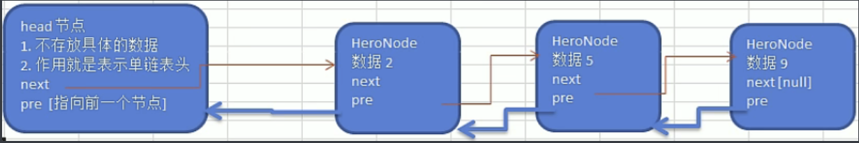
2. 双链表
-
单链表存在的问题
- 单向链表查找的方向只能是一个方向(即头节点往后),而双向链表可以向前或者向后查找。
- 单向链表不能自我删除,需要借助辅助节点,而双向链表可以自我删除
-
示意图
-
处理方法
-
遍历和单链表一样,只是多了一个
pre指针,可以双向遍历(向前向后查找) -
添加节点,将节点的两个指针连在双向链表最后一个节点即可
-
修改节点,先遍历找到节点,然后改变其值
-
删除节点,先便利找到这个节点
temp,将前节点的next指针指向后节点,后节点的pre指针指向前节点(此处可以temp.pre.next=temp.next&&temp.next.pre=temp.pre) -
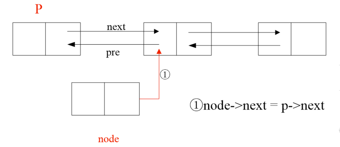
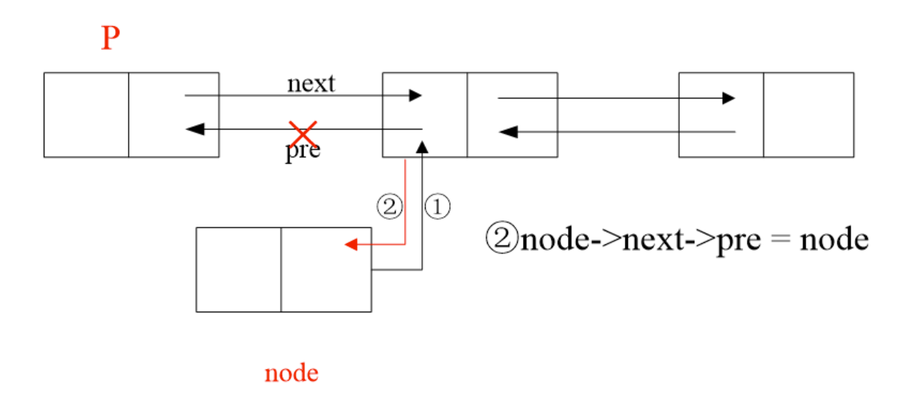
按顺序插入节点,先确定插入位置,然后插入,原理如下图(分四步,顺序不能乱)
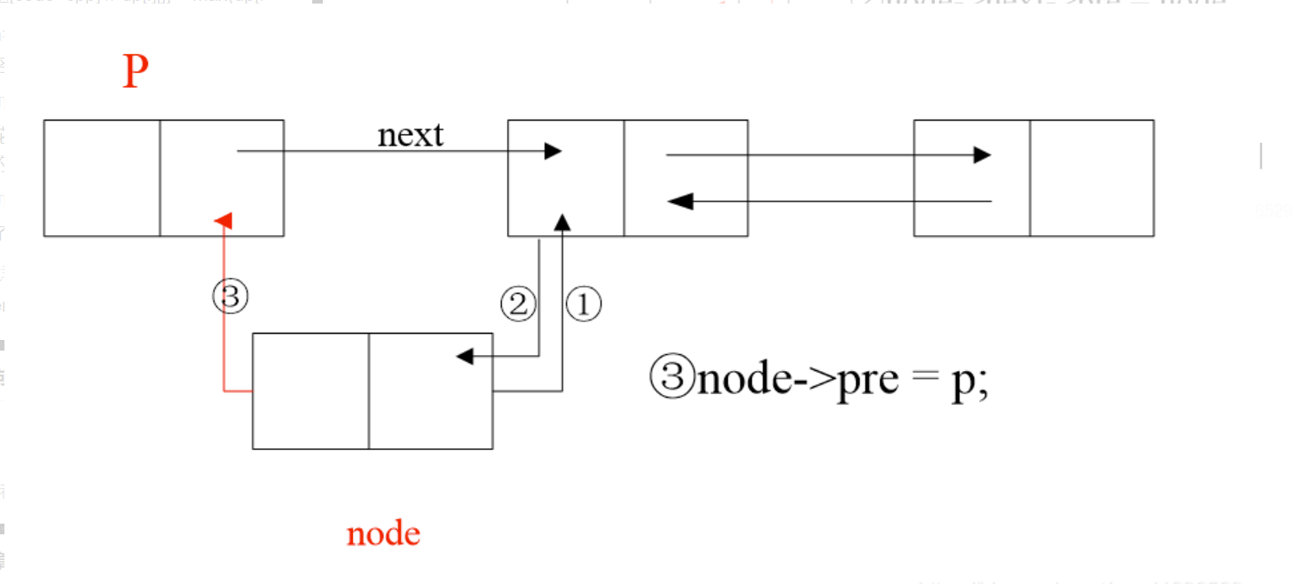
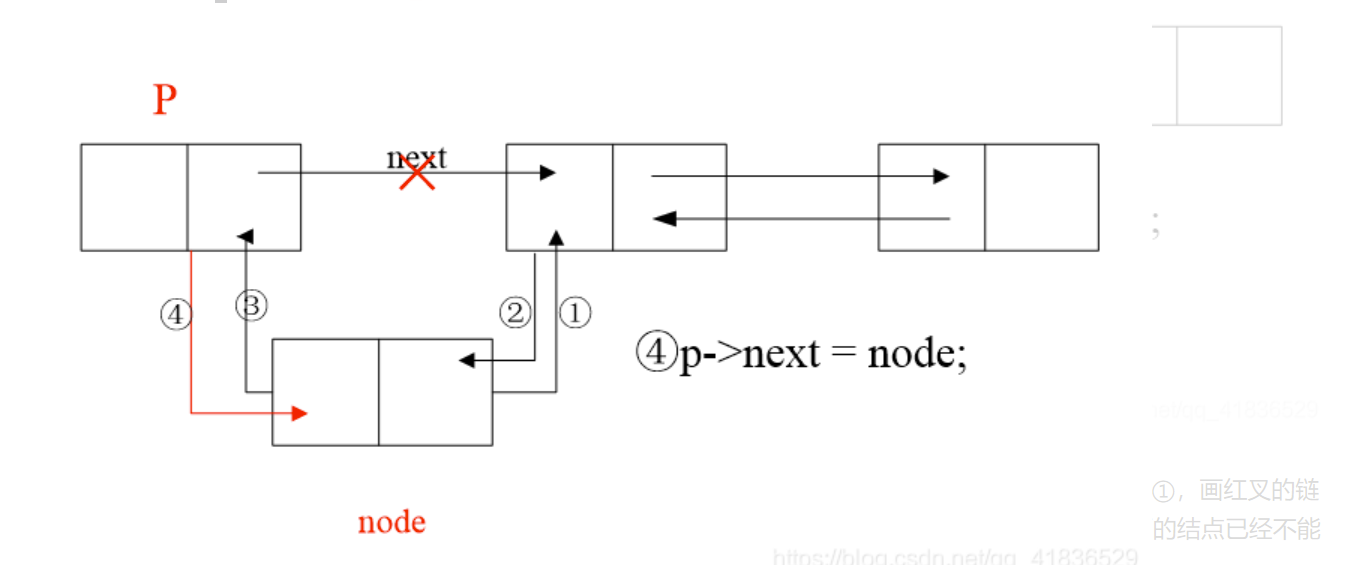
-
-
代码实现
  1
  2
  3
  4
  5
  6
  7
  8
  9
 10
 11
 12
 13
 14
 15
 16
 17
 18
 19
 20
 21
 22
 23
 24
 25
 26
 27
 28
 29
 30
 31
 32
 33
 34
 35
 36
 37
 38
 39
 40
 41
 42
 43
 44
 45
 46
 47
 48
 49
 50
 51
 52
 53
 54
 55
 56
 57
 58
 59
 60
 61
 62
 63
 64
 65
 66
 67
 68
 69
 70
 71
 72
 73
 74
 75
 76
 77
 78
 79
 80
 81
 82
 83
 84
 85
 86
 87
 88
 89
 90
 91
 92
 93
 94
 95
 96
 97
 98
 99
100
101
102
103
104
105
106
107
108
109
110
111
112
113
114
115
116
117
118
119
120
121
122
123
124
125
126
127
128
129
130
131
132
133
134
135
package linkedList; public class doublyLinkedList { public static void main(String[] args) { heroNode1 h1 = new heroNode1(1, "刘海斌"); heroNode1 h2 = new heroNode1(2, "包文杰"); heroNode1 h3 = new heroNode1(3, "王铁霖"); heroNode1 h4 = new heroNode1(4, "牟国柱"); managerHeroNode1 m =new managerHeroNode1(); m.addNode(h1); m.addNode(h2); m.addNode(h3); m.addNode(h4); m.listNode(); m.updateNode(new heroNode1(2,"小包")); m.insertNode(new heroNode1(3,"邓涔浩")); m.deleteNode(4); m.listNode(); } } class managerHeroNode1 { heroNode1 head; public managerHeroNode1() { this.head = new heroNode1(-1, ""); } public boolean isEmpty() { if (head.next != null) return false; else return true; } //末尾添加node public void addNode(heroNode1 node) { heroNode1 temp = head; //遍历到末尾 while (temp.next != null) { temp = temp.next; } temp.next = node; node.pre = temp; System.out.println("成功添加"); } //修改节点 public void updateNode(heroNode1 node) { if (isEmpty()) { System.out.println("链表为空"); return; } heroNode1 temp = head; while (temp.no != node.no) { temp = temp.next; if (temp == null) { System.out.println("没找到该节点"); return; } } temp.name = node.name; System.out.println("修改成功:" + temp); } //删除节点 public void deleteNode(int no) { if (isEmpty()) { System.out.println("链表为空"); return; } heroNode1 temp = head; while (temp.no != no) { temp = temp.next; } //temp的下一个节点的pre指针指向temp的上一个节点 // temp.next.pre=temp.pre;//注意如果temp是最后一个节点,这里有错: if (temp.next != null) temp.next.pre = temp.pre; //temp的上一个节点的next指针指向temp的下一个节点 temp.pre.next = temp.next; System.out.println("删除成功:" + temp); } //按序插入节点 public void insertNode(heroNode1 node) { if (isEmpty()) { System.out.println("链表为空"); return; } heroNode1 temp = head; while (temp.no <= node.no) { temp = temp.next; //如果插入节点在最后,直接添加 if (temp==null){ addNode(node); return; } } //此操作注意先后顺序,否则会因为链条一部分断裂而导致后面的节点变成null //首先 node.pre=temp; node.next=temp.next; temp.next=node; temp.next.pre=node; System.out.println("插入成功:" + node); } //遍历链表 public void listNode() { if (isEmpty()) { System.out.println("链表为空"); return; } heroNode1 temp = head; while (temp.next != null) { temp = temp.next; System.out.println(temp); } } } class heroNode1 { //节点data属性 int no; String name; //指针域 heroNode1 pre; heroNode1 next; public heroNode1(int no, String name) { this.no = no; this.name = name; } @Override public String toString() { return "heroNode1{" + "no=" + no + ", name='" + name + '\'' + '}'; } }
3. 单向环形链表
-
原理
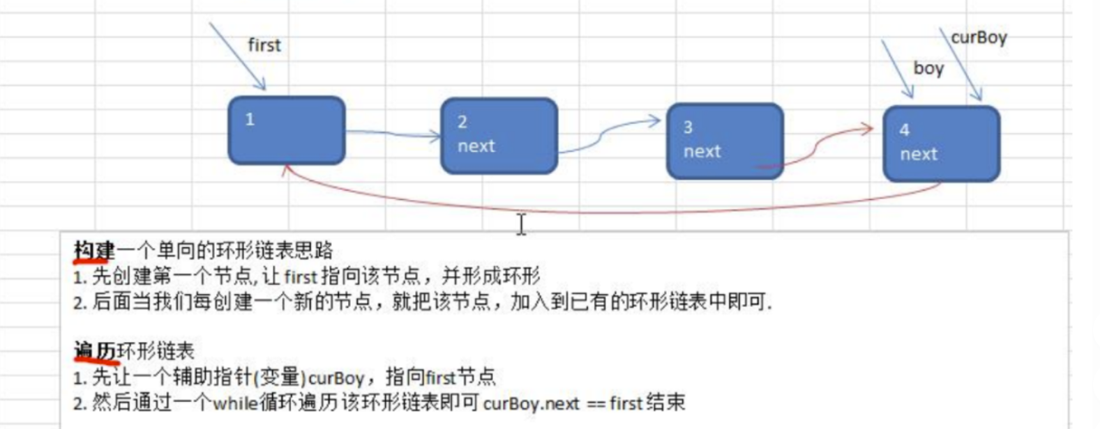
-
约瑟夫问题
在罗马人占领乔塔帕特后,39个犹太人和Josephus及他的朋友躲进一个洞里,39个犹太人决定宁愿死也不要被敌人抓到,于是决定了一个自杀方式,41个人排成一个圆圈,由第一个人开始报数,报数到3的人就自杀,再由下一个人重新报1,报数到3的人就自杀,这样依次下去,知道剩下最后一个人时,那个人可以自由选择自己的命运。这就是著名的约瑟夫问题。现在请用单向链表描述该结构并呈现整个自杀过程。
单向环形链表解决
-
代码实现
  1
  2
  3
  4
  5
  6
  7
  8
  9
 10
 11
 12
 13
 14
 15
 16
 17
 18
 19
 20
 21
 22
 23
 24
 25
 26
 27
 28
 29
 30
 31
 32
 33
 34
 35
 36
 37
 38
 39
 40
 41
 42
 43
 44
 45
 46
 47
 48
 49
 50
 51
 52
 53
 54
 55
 56
 57
 58
 59
 60
 61
 62
 63
 64
 65
 66
 67
 68
 69
 70
 71
 72
 73
 74
 75
 76
 77
 78
 79
 80
 81
 82
 83
 84
 85
 86
 87
 88
 89
 90
 91
 92
 93
 94
 95
 96
 97
 98
 99
100
package linkedList; public class singleRingLinkedList { public static void main(String[] args) { managerList m = new managerList(); m.addNode(41); m.list(); System.out.println(); m.pops(1, 3, 5); } } class managerList { boyNode head; public managerList() { //头节点,标记首位置 head = new boyNode(-1); head.next = head;//注意闭环 } //添加 public void addNode(int num) { if (num < 1) { System.out.println("参数错误"); return; } boyNode curNode = head; for (int i = 1; i <= num; i++) { boyNode node = new boyNode(i); if (i == 1) { head.no = node.no; continue; } curNode.next = node; node.next = head; //记录当前节点 curNode = node; } System.out.println("添加成功"); } //遍历链表 public void list() { if (head == null) { System.out.println("链表为空"); return; } boyNode curNode = head; while (curNode.next != head) { System.out.println(curNode); curNode = curNode.next; } System.out.println(curNode); } //取出节点 public void pops(int startNo, int countNum, int nums) { //先对数据进行检验 if (head==null||countNum<1||countNum>nums){ System.out.println("参数输入有误"); return; } //helper指针指向链表尾节点 boyNode helper = head; while (helper.next != head) { helper = helper.next; } //移动到报数节点 for (int i = 0; i < startNo-1; i++) { helper = helper.next; head = head.next; } while (head != helper) { //报数移动countNum-1次 for (int i = 1; i < countNum; i++) { helper = helper.next; head = head.next; } int number = head.no; head = head.next; helper.next = head; System.out.println("移除节点:" + number); } System.out.println("最后的节点:" + head.no); } } class boyNode { int no;//编号 boyNode next;//指针域 public boyNode(int no) { this.no = no; } @Override public String toString() { return "boyNode{" + "no=" + no + '}'; } }
四、栈
1. 原理
-
栈是一个先入后出的有序列表
-
栈是限制线性表中元素的插入和删除只能在线性表的同一端进行的一种特殊线性表。允许插入和删除的一端,为变化的一端,称为栈顶;另一端为固定的一端,成为栈底
-
最先放入栈的元素在栈底,最后放入的元素在栈顶;而删除元素刚好相反,最后放入的元素最先删除,最先放入的元素最后删除
-
原理图
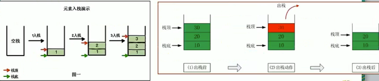
2. 代码实现(数组模拟栈)
|
|
3. 波兰计算器
① 无括号版波兰计算器
-
思路
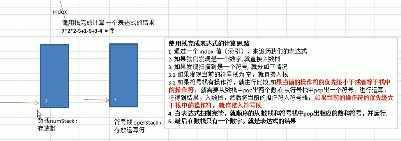
针对多位数运算时的逻辑:如果扫描到数字就继续扫描下一位直到不是数字为止,将扫描的数字字符拼接成串然后转化为数字
-
代码实现
1 2 3 4 5 6 7 8 9 10 11 12 13 14 15 16 17 18 19 20 21 22 23 24 25 26 27 28 29 30 31 32 33 34 35 36 37 38 39 40 41 42 43 44 45 46 47 48 49 50 51 52 53 54 55 56 57 58 59 60 61 62 63 64 65 66 67 68 69 70 71 72 73 74 75 76 77 78 79 80 81 82 83 84 85 86 87 88 89 90 91 92 93 94 95 96 97 98 99 100 101 102 103 104 105 106 107 108 109 110 111 112 113 114 115 116 117 118 119 120 121 122 123 124 125 126 127package stack; import java.util.Scanner; public class calculatorByStackDemo { public static void main(String[] args) { Scanner sc = new Scanner(System.in); System.out.print("请输入合法表达式:"); String express = sc.next(); char[] chars = express.toCharArray(); //数字栈 stack stackNumber = new stack(10); //符号栈 stack stackOperation = new stack(10); int num1 = 0; int num2 = 0; int val = 0; int operation = 0; String number = ""; for (int i = 0; i < chars.length; ) { //符号 if (stackOperation.isOperation(chars[i])) { //符号栈为空,将符号压入符号栈 if (stackOperation.isEmpty()) stackOperation.push(chars[i]); else if (!stackOperation.isFull()) { //如果符号栈有操作符,进行比较,如果当前操作符的优先级低于或等于栈中的操作符, //就需要从数栈中pop两个数,再从符号栈里pop出一个符号进行运算,将得到的结果压 //入数栈,然后再将当前的操作符压入符号栈中 if (stackOperation.priority(chars[i]) <= stackOperation.priority(stackOperation.showTop())) { num1 = stackNumber.pop(); num2 = stackNumber.pop(); operation = stackOperation.pop(); val = stackNumber.calculate(num2, num1, operation); stackNumber.push(val); stackOperation.push(chars[i]); } else { //当前操作符优先级更高,再压入符号栈中 stackOperation.push(chars[i]); } } i++; } //如果是数字,先别慌入栈,再判断下一位是否是数字,是数字就拼接在一起 // if (stackNumber.isDigital(chars[i])){ // stackNumber.push(Character.getNumericValue(number)); // } while (stackNumber.isDigital(chars[i])) { number = number + chars[i]; i++; if (i == chars.length) break; } System.out.println(number); stackNumber.push(Integer.parseInt(number)); number = "";//清空上次数字残余 } //扫描完毕后,顺序从数栈和符号栈pop出两个数字和一个符号,并运算,最后数栈只有一个数字就是结果 //最后的栈中运算符都是同等优先级的运算符 while (!stackOperation.isEmpty()) { num1 = stackNumber.pop(); num2 = stackNumber.pop(); operation = stackOperation.pop(); val = stackOperation.calculate(num2, num1, operation); stackNumber.push(val); } System.out.println("计算的结果是:" + stackNumber.showButton()); } } class stack { int top; int maxSize; int[] nodes; public stack(int maxSize) { top = -1; this.maxSize = maxSize; nodes = new int[maxSize]; } public boolean isEmpty() { return top == -1; } public boolean isFull() { return top == maxSize - 1; } //入栈 public void push(int node) { if (isFull()) throw new RuntimeException("栈溢出"); nodes[++top] = node; } //出栈 public int pop() { if (isEmpty()) throw new RuntimeException("栈空"); return nodes[top--]; } //显示栈顶元素,但不取出 public int showTop() { return nodes[top]; } public int showButton() { return nodes[0]; } //优先级 public int priority(int operation) { if (operation == '*' || operation == '/') return 1; else if (operation == '+' || operation == '-') return 0; return -1; } //判断是不是操作符 public boolean isOperation(int operation) { return operation == '+' || operation == '-' || operation == '*' || operation == '/'; } //判断是不是数字 public boolean isDigital(int number) { return Character.isDigit(number); } //计算方法 public int calculate(int num1, int num2, int operation) { switch (operation) { case '+': return num1 + num2; case '-': return num1 - num2; case '*': return num1 * num2; case '/': return num1 / num2; default: return 0; } } }
② 前缀表达式(波兰表达式)
- 前缀表达式的运算符位于操作数之前。如
(3+4)*5-6这样的中缀表达式对应的前缀表达式-*+3456 - 前缀表达式的计算机求值:首先从右至左扫描表达式,遇到数字则将数字压入堆栈,遇到运算符则弹出栈顶的两个数字,用运算符对这两数字做运算,并将结果再次入栈,重复上述过程直至表达式最左端,最后数栈的里的最后一个元素就是该表达式的值。
③ 中缀表达式
- 中缀表达式是常见的运算表达式,如
(3+4)*5-6 - 中缀表达式的求值是对人类友好的,但是计算机不好理解,在计算机求解过程中往往会将中缀表达式转化为其他表达式来操作(一般往往是后缀表达式,因为中缀表达式的操作符顺序不好确定)
④ 后缀表达式(逆波兰表达式)
- 与前缀表达式相反,后缀表达式的运算符位于操作数之后,如
(3+4)*5-6这样的中缀表达式对应的后缀表达式34+5*6- - 后缀表达式的计算机求值,与前缀表达式相反:首先从左至右扫描表达式,遇到数字则将数字压入堆栈,遇到运算符则弹出栈顶的两个数字,用运算符对这两数字做运算,并将结果再次入栈,重复上述过程直至表达式最左端,最后数栈的里的最后一个元素就是该表达式的值。
4. 逆波兰计算器
① 后缀表达式求解
求解思路如上
|
|
该实例演示了对后缀表达式进行计算求解。但是用户往往是输入中缀表达式。以下代码,实现利用中缀表达式转化为后缀表达式,然后再通过以上方法再求解后缀表达式。
② 中缀表达式转化为后缀表达式
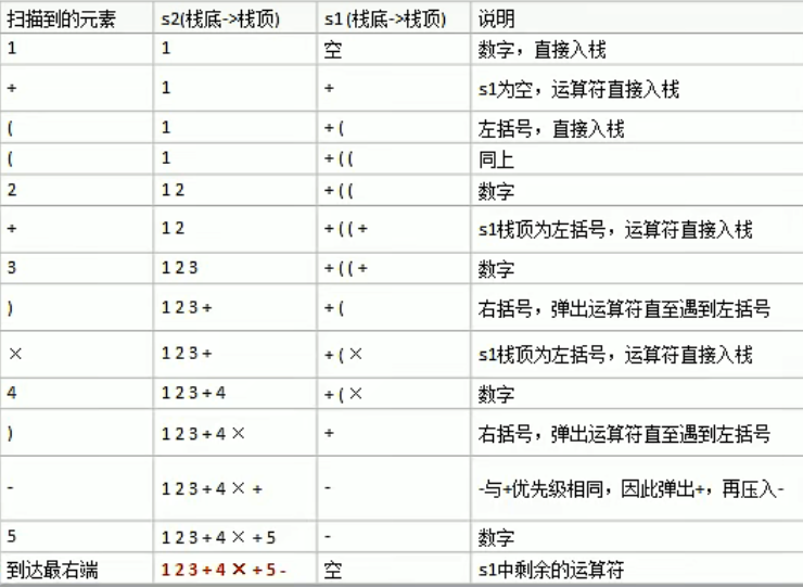
思路(注意各个步骤顺序):
- 初始化两个栈:运算符栈s1和储存中间结果栈s2
- 从左至右扫描中缀表达式
- 遇到操作数时,将其压入栈s2
- 遇到括号时:如果是左括号“(”,则直接入栈;如果是右括号“)”,则依次弹出s1栈顶的运算符,并压入到s2中,直到遇到左括号为止,此时将这一对括号丢弃
- 遇到运算符时,比较其与s1栈顶运算符的优先级:如果s1为空或栈顶运算符为左括号“(”,再或者优先级比栈顶的运算符的高,就将运算符压入s1栈中;否则(不满足前面三个条件之一),即优先级比栈顶运算符的低或相等,将s1栈顶运算符弹出并压入到s2中,再次转到第四步开始重新比较当前运算符
- 重复步骤2-5,直至表达式地最右边
- 将s1剩余地运算符依次弹出并压入s2
- 依次弹s2中的元素并输出结果,结果的逆序极为中缀表达式对应的后缀表达式。
样例分析
中缀表达式:1+((2+3)*4)-5
后缀表达式结果:1 2 3 + 4* + 5 -
代码展示
|
|
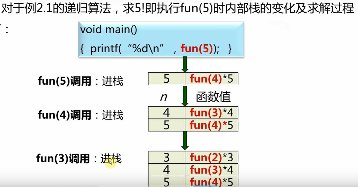
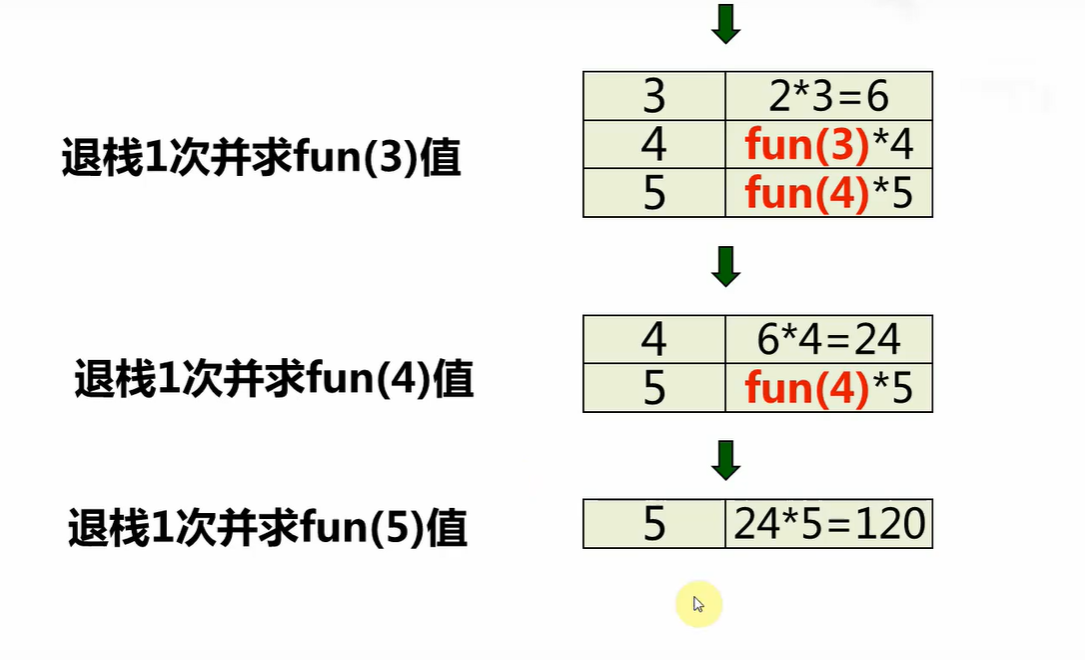
5. 递归
① 原理
递归,就是在运行的过程中调用自己。
构成递归需具备的条件
- 构成递归需具备的条件
- 不能无限制地调用本身,须有个出口,化简为非递归状况处理
② 递归机制
- 进栈:每递归调用一次函数或方法,就需要进栈一次,最多的进栈元素个数称为递归深度,递归次数越多,递归深度越大,开辟的栈空间越大(应当避免过多的递归使得栈溢出)
- 出栈:每当遇到递归出口或**完成本次执行(完成执行的意思:执行函数或方法到达底部)**时,需出栈一次并恢复参量值,当全部执行完毕时,栈应为空。
- 为了完成一次典型的递归调用,系统需要分配一些空间来保存三部分重要的信息
- 函数的返回地址:一旦函数调用完成,程序应该知道返回到哪里,即函数调用之前的位置
- 函数传递的参数
- 函数的局部变量
- 每次进行递归调用时,都会在栈中有自己的形参和局部变量的拷贝,这个由系统自动完成,即将所有的栈变量压入系统的堆栈。(如果是浅拷贝形参则每个方法或函数压入栈的变量都是相互独立的;但是如果是深拷贝,则会互相影响)
- 由于有了a)的机制,在递归返回的时候才能将前面压入栈的临时变量又恢复到现场
④ 递归示例图

⑤ 递归应用
- 各种数学问题:八皇后、汉诺塔、阶乘、迷宫等
- 各种算法也会使用递归,比如快排、归并排序、二分查找、分治算法等
- 利用栈解决的问题-》递归代码比较简洁
迷宫回溯
如下图,红色方块代表墙,红色圆形代表小球,小球在指定起点位置需要寻找一条到达指定目的地的最短路径
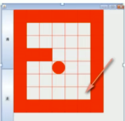
思路
- 初始化地图,假设有墙的地方值为1;没有墙可以走的地方值为0;走过点设置为2;已经探测过没有后路的点设置为3
- 定制策略,有上下左右四个方向,因此策略有24种策略。只需要找到哪种策略的2的点数最少到达目的地即可
代码实现
|
|
八皇后(回溯算法)
在8*8格的国际象棋上拜访八个皇后,使其不能相互攻击,即:任意两个皇后都不能处于同一行、同一列或同一斜线上,问有多少种摆法?(答案:92种)
思路(暴力法)
- 第一个皇后先放第一列
- 第二个皇后放在第二行第一列,然后判断是否ok,如果不ok,继续放在第二列、第三列,依次把所有的列放完,找到一个合适的位置
- 继续第三个皇后,还是第一列、第二列…直到第八个皇后也能放在一个不冲突的位置,于是就找到了一个正确解
- 当得到一个正确解时,在栈回退到上一个栈时,就会开始回溯,即将第一个皇后放到第一列的所有正确解全部得到
- 然后回头继续第一个皇后放到第二列,后面依次循环执行1、2、3、4的步骤
说明:理论上应该创建一个二维数组来表示棋盘地图,但是实际上可以通过算法用一个一维数组解决问题,如int[] arr = new int[]{0,4,7,5,2,6,1,3} arr数组下标表示第几行,即第几个皇后,值表示列的位置:arr[i]表示第i+1个皇后,放在第i+1行的第arr[i]+1列。当然也可以使用二维数组实现,但是
代码实现
|
|
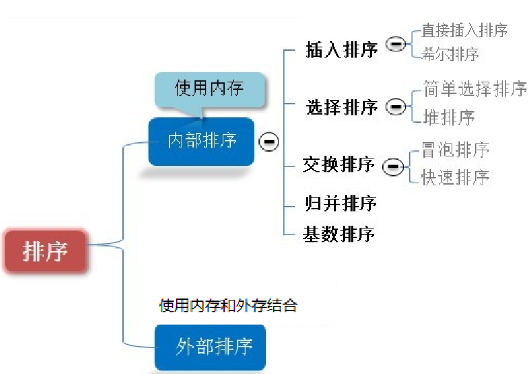
五、排序算法
排序也称排序算法,排序是将一组数据依指定顺序进行排列的过程。
排序的分类:
-
内部排序
指将需要处理的所有数据都加载到内部存储器中进行排序。
-
外部排序
数据量过大,无法全部加载到内存中,需要借助外部存储进行排序
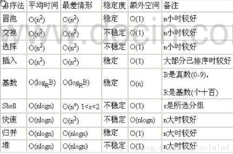
常见的排序算法分类
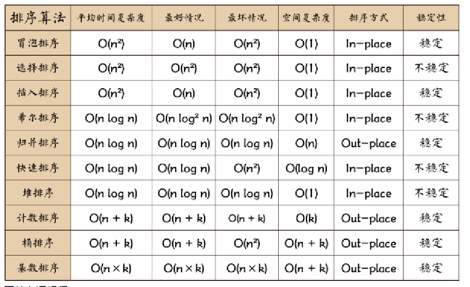
相关术语:
- 稳定:如果a原本在b前面,而a=b,排序之后a仍然在b的前面;
- 不稳定:如果a原本在b的前面,而a=b,排序之后a可能会出现在b的后面;
- 内排序:所有排序操作都在内存中完成;
- 外排序:由于数据太大,因此把数据放在磁盘中,而排序通过磁盘和内存的数据传输才能进行;
- 时间复杂度: 一个算法执行所耗费的时间。
- 空间复杂度:运行完一个程序所需内存的大小。
- n: 数据规模
- k: “桶”的个数,不做特殊的处理的话,一般为10
- In-place: 不占用额外内存
- Out-place: 占用额外内存
1. 冒泡排序
-
原理
通过对待排序序列从前往后(从下标较小的元素开始),依次比较相邻元素的值,若发现逆序则交换,使值较大。
算法复杂度:
O()
-
算法描述
- 比较相邻的元素。如果第一个比第二个大,就交换它们两个
- 对每一对相邻元素作同样的工作,从开始第一对到结尾的最后一对,这样在最后的元素应该会是最大的数,同时这个元素也是排好序的元素
- 针对所有的元素重复以上的步骤,除了最后一个
- 重复步骤1~3,直到排序完成
- 优化:因为排序的过程中,各元素不断接近自己的位置,如果一趟比较下 来没有进行过交换,就说明序列已经有序,无需再比较下去
-
代码实现
1 2 3 4 5 6 7 8 9 10 11 12 13 14 15 16 17 18 19 20 21 22 23 24 25 26 27 28 29 30 31 32package sort; import java.util.Arrays; /* * 冒泡排序 * */ public class bubbleSort { public static void main(String[] args) { int[] arr = new int[]{1, 2, 1, 5, 4, 6, 4, 1}; System.out.println(Arrays.toString(arr)); bubbleSort(arr); System.out.println(Arrays.toString(arr)); } public static void bubbleSort(int[] arr) { int temp = 0; boolean flag = false; for (int i = 0; i < arr.length - 1; i++) {//需要多少轮两两比较,每一轮都会选出一个排好序的数字 flag = false; for (int j = 0; j < arr.length - 1 - i; j++) { // 从第一个元素到第i个元素 if (arr[j] > arr[j + 1]) { //交换值 temp = arr[j]; arr[j] = arr[j + 1]; arr[j + 1] = temp; flag = true; } } if (!flag) { break; } } } }
2. 选择排序
-
原理
选择排序是一种简单直观的排序算法,它也是一种交换排序算法,和冒泡排序有一定的相似度,可以认为选择排序是冒泡排序的一种改进
-
算法描述
- 在未排序序列中找到最小(大)元素,存放到排序序列的起始位置
- 从剩余未排序元素中继续寻找最小(大)元素,然后放到已排序序列的末尾
- 重复第二步,直到所有元素均排序完毕
-
代码实现
1 2 3 4 5 6 7 8 9 10 11 12 13 14 15 16 17 18 19 20 21 22 23 24 25 26 27 28 29 30 31package sort; import java.util.Arrays; /* * 选择排序 * */ public class selectionSort { public static void main(String[] args) { int[] arr = new int[]{1, 2, 1, 5, 4, 6, 4, 1}; System.out.println(Arrays.toString(arr)); selectionSort(arr); System.out.println(Arrays.toString(arr)); } public static void selectionSort(int[] arr) { int temp, min, index = 0; for (int i = 0; i < arr.length - 1; i++) { min = arr[i];//最小值 for (int j = i + 1; j < arr.length; j++) {//从i的下一个元素开始到最后一个元素进行比较 if (min > arr[j]) { min = arr[j]; index = j;//记录最小值角标 } } if (min != arr[i]) {//min值改变,说明找到更小的值,需要交换 temp = arr[i]; arr[i] = arr[index]; arr[index] = temp; } } } }
3. 插入排序
-
原理
插入排序是一种简单直观的排序算法。它的工作原理是通过构建有序序列,对于未排序数据,在已排序序列中从后向前扫描,找到相应位置并插入
-
算法描述
-
把待排序的数组分成已排序和未排序两部分,初始的时候把第一个元素认为是已排好序的
-
从第二个元素开始,在已排好序的子数组中寻找到该元素合适的位置并插入该位置
-
重复上述过程直到最后一个元素被插入有序子数组中
-
问题
1 2 3 4 5 6 7 8 9我们看简单的插入排序可能存在的问题. 数组 arr = {2,3,4,5,6,1} 这时需要插入的数 1(最小), 这样的过程是: {2,3,4,5,6,6} {2,3,4,5,5,6} {2,3,4,4,5,6} {2,3,3,4,5,6} {2,2,3,4,5,6} {1,2,3,4,5,6} 结论: 当需要插入的数是较小的数时,后移的次数明显增多,对效率有影响
-
-
代码实现
1 2 3 4 5 6 7 8 9 10 11 12 13 14 15 16 17 18 19 20 21 22 23 24 25 26 27 28 29 30 31 32 33 34 35 36 37 38 39package sort; import java.util.Arrays; /* * 插入排序 */ public class insertionSort { public static void main(String[] args) { int[] arr = new int[]{1, 2, 1, 5, 4, 6, 4, 1}; System.out.println(Arrays.toString(arr)); insertionSort(arr); System.out.println(Arrays.toString(arr)); } public static void insertionSort(int[] arr) { // for (int i = 1; i < arr.length; ++i) { // int value = arr[i];//记录当前需要比较的数据 // int position = i;//记录当前数据角标 // while (position > 0 && arr[position - 1] > value) {//大于value的素数组元素往后挪一位,直到不大于 // arr[position] = arr[position - 1]; // position--; // } // arr[position] = value; // } for (int i = 1; i < arr.length; i++) { int val = arr[i]; int index = i; for (; index > 0; index--) { if (arr[index - 1] > val) { arr[index] = arr[index - 1]; } else { break; } } arr[index] = val; } } }
4. 希尔排序
-
原理
移位法思路:
希尔排序也是一种插入排序,它是简单插入排序经过改进之后的一个更高效的版本,也称为缩小增量排序。希尔排序是记录下标的一定增量分组,对每组使用直接插入排序算法排序;随着增量逐渐减少,每组包含的关键词越来越多,当增量减至1时,整个文件恰被分成一组,算法便终止。增量序列的选取:希尔增量、Hibbard增量、Sedgewick增量
-
算法描述
先将整个待排序的记录序列分割成为若干子序列分别进行直接插入排序,具体算法描述:
- 选择一个增量序列t1,t2,…,tk,其中ti>tj,tk=1
- 按增量序列个数k,对序列进行 k 趟排序
- 每趟排序,根据对应的增量ti,将待排序列分割成若干长度为m 的子序列,分别对各子表进行直接插入排序。仅增量因子为1 时,整个序列作为一个表来处理,表长度即为整个序列的长度
-
代码实现(选用希尔增量)
交换法
1 2 3 4 5 6 7 8 9 10 11 12 13 14 15 16 17 18 19 20 21 22 23 24 25 26 27 28package sort; import java.util.Arrays; /* * 希尔排序(交换法) */ public class shellSort { public static void main(String[] args) { int[] arr = new int[]{1, 2, 1, 5, 4, 6, 4, 1}; System.out.println(Arrays.toString(arr)); shellSort(arr); System.out.println(Arrays.toString(arr)); } public static void shellSort(int[] arr) { int temp; for (int gap = arr.length / 2; gap > 0; gap /= 2) {//增量序列,gap为步长,分组 for (int i = 0; i < arr.length - gap; i++) {//遍历有多少组:(arr.length-gap)组 for (int j = 0; j < arr.length - gap; j += gap) {//遍历交换组内元素 if (arr[j] > arr[j + gap]) { temp = arr[j]; arr[j] = arr[j + gap]; arr[j + gap] = temp; } } } } } }注意:交换法对数据进行排序,在数据量大的时候,变得很慢。采用移动法进行优化
移位法
1 2 3 4 5 6 7 8 9 10 11 12 13 14 15 16 17 18 19 20 21 22 23 24 25 26 27 28 29package sort; import java.util.Arrays; public class shellSort { public static void main(String[] args) { int[] arr = new int[]{1, 2, 1, 5, 4, 6, 4, 1}; System.out.println("排序前:" + Arrays.toString(arr)); shellSortByMove(arr); System.out.println("移位法排序后:" + Arrays.toString(arr)); } public static void shellSortByMove(int[] arr) { for (int gap = arr.length / 2; gap > 0; gap /= 2) {//分组 //对每组所有元素进行直接插入排序 for (int i = gap; i < arr.length; i++) { int position = i; int value = arr[i]; if (value < arr[position - gap]) { while (position - gap >= 0 && value < arr[position - gap]) { arr[position] = arr[position - gap]; position -= gap; } arr[position] = value; } } } } }
5. 快速排序
-
原理
快速排序(Quicksort)是对冒泡排序的一种改进。基本思想是:通过一趟排序将要排序的数据分割成独立的两部分,其中一部分的所有数据都比另外一部分的所有数据都要小,然后再按此方法对这两部分数据分别进行快速排序,整个排序过程可以递归进行,以此达到整个数据变成有序序列
-
算法描述
- 从数列中挑出一个元素,称为"基准"(pivot)
- 重新排序数列,所有比基准值小的元素摆放在基准前面,所有比基准值大的元素摆在基准后面(相同的数可以到任何一边)。在这个分区结束之后,该基准就处于数列的中间位置。这个称为分区(partition)操作
- 递归地(recursively)把小于基准值元素的子数列和大于基准值元素的子数列排序
-
代码实现
1 2 3 4 5 6 7 8 9 10 11 12 13 14 15 16 17 18 19 20 21 22 23 24 25 26 27 28 29 30 31 32 33 34 35 36 37 38 39package sort; import java.util.Arrays; public class quickSort { public static void main(String[] args) { int[] arr = new int[]{1, 2, 1, 5, 4, 6, 4, 1}; // int[] arr = new int[]{-9,78,0,23,-567,70}; System.out.println("排序前:" + Arrays.toString(arr)); quickSort(arr); System.out.println("排序后:" + Arrays.toString(arr)); } public static void quickSort(int[] arr) { qsort(arr, 0, arr.length - 1); } private static void qsort(int[] arr, int low, int high) { if (low >= high) return; int pivotIndex = partition(arr, low, high); //将数组分为两部分 qsort(arr, low, pivotIndex - 1); //递归排序左子数组 qsort(arr, pivotIndex + 1, high); //递归排序右子数组 } private static int partition(int[] arr, int low, int high) { int pivot = arr[low]; //记录基准 while (low < high) { while (low < high && arr[high] >= pivot) --high; arr[low] = arr[high]; //交换比基准小的记录到左端low角标处 while (low < high && arr[low] <= pivot) ++low; arr[high] = arr[low]; //交换比基准大的记录到右端high角标处 } //扫描完成,基准移到新的基准 arr[low] = pivot; //返回的是新基准的位置 return low; } }
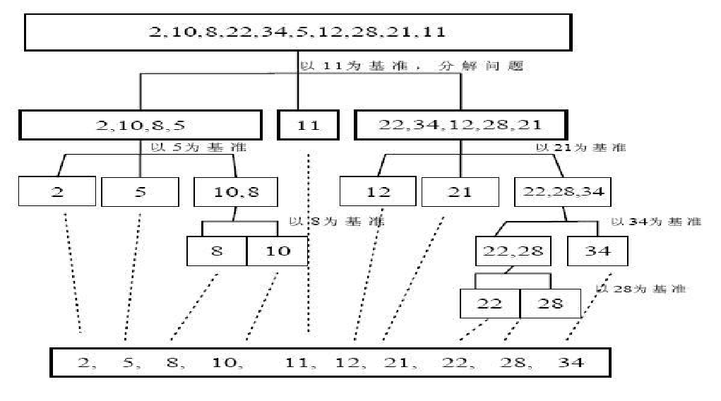
6. 归并排序
-
原理
归并排序是利用归并的思想实现的排序方法,该算法采用经典的分治策略(分治法将问题分成一些小的问题然后递归求解,而治的阶段则将分的阶段得到的各答案“修补”在一起,即分而治之)
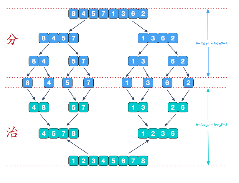
说明:可以看到这种结构很像一棵完全二叉树,本文的归并排序我们采用递归去实现(也可采用迭代的方式去实现)。分阶段可以理解为就是递归拆分子序列的过程。
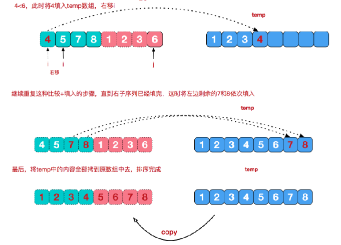
再来看看治阶段,我们需要将两个已经有序的子序列合并成一个有序序列,比如上图中的最后一次合并,要将
[4,5,7,8]和[1,2,3,6]两个已经有序的子序列,合并为最终序列[1,2,3,4,5,6,7,8],来看下实现步骤(双指针法)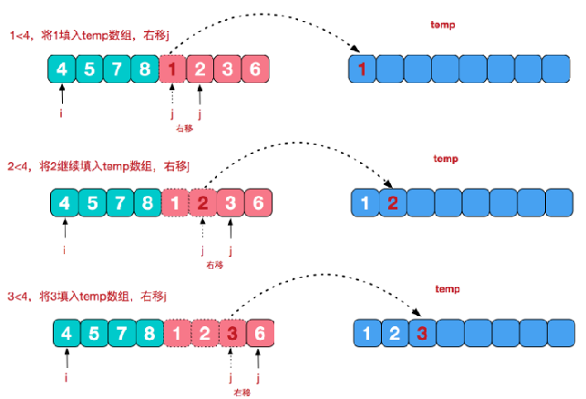
-
代码实现
1 2 3 4 5 6 7 8 9 10 11 12 13 14 15 16 17 18 19 20 21 22 23 24 25 26 27 28 29 30 31 32 33 34 35 36 37 38 39 40 41 42 43 44 45 46 47 48 49 50 51 52 53 54 55 56 57 58 59package sort; import java.util.Arrays; public class mergeSort { public static void main(String[] args) { int[] arr = {8, 4, 5, 7, 1, 3, 6, 2}; // int[] arr = {4, 5, 7, 8, 1, 2, 3, 6}; int[] temp = new int[arr.length]; System.out.println("排序前:" + Arrays.toString(arr)); mergeSort(arr, 0, arr.length - 1, temp); System.out.println("排序后:" + Arrays.toString(arr)); } //分+和 public static void mergeSort(int[] arr, int left, int right, int[] temp) { if (left < right) { int mid = (left + right) / 2;//中间索引 //向左递归分解 mergeSort(arr, left, mid, temp); //向右递归分解 mergeSort(arr, mid + 1, right, temp); //合并 merge(arr, left, mid, right, temp); } } //mid指左子序列最后一个元素 public static void merge(int[] arr, int left, int mid, int right, int[] temp) { int i = left;//指左子序列起点处 int j = mid + 1;//指右子序列起点处 int t = 0;//temp数组索引 //先将左右两边有序数据填充到temp数组,直到又一边填充完毕 while (i <= mid && j <= right) { if (arr[i] <= arr[j]) { temp[t] = arr[i]; t++; i++; } else if (arr[i] > arr[j]) { temp[t] = arr[j]; t++; j++; } } //再将一边剩下的有序数据移到temp后面 while (i <= mid) { temp[t++] = arr[i++]; } while (j <= right) { temp[t++] = arr[j++]; } //拷贝指定数量至arr数组,注意左右拷贝边界 t = 0; int tLeft = left; while (tLeft <= right) { arr[tLeft++] = temp[t++]; } } }
7. 基数排序
-
原理
基数排序(
radix sort)属于“分配式排序”,又称“桶子法”,顾名思义,它是通过键值的各个位的值,将要排序的元素分配至某些“桶”中,达到排序的作用。基数排序法是属于稳定性的排序,基数排序法的是效率高的稳定性排序法。基数排序是桶排序的扩展。基数排序是这样实现的:将整数按位数切割成不同的数字,然后按每个位数分别比较。注:假定在待排序的记录序列中,存在多个具有相同的关键字的记录,若经过排序,这些记录的相对次序保持不变,即在原序列中,
r[i]=r[j],且r[i]在r[j]之前,而在排序后的序列中,r[i]仍在r[j]之前,则称这种排序算法是稳定的;否则称为不稳定的**有负数的数组,我们不用基数排序来进行排序, 如果要支持负数,参考: https://code.i-harness.com/zh-CN/q/e98fa9 **
-
算法实现
将所有待比较数值统一为同样的数位长度,数位较短的数前面补零。然后,从最低位开始,依次进行一次排序,相同的数放到同一个“桶”(数组),然后再依次从“桶”中取出元素,形成的序列再比较各个数字下一位,这样从最低位排序一直到最高位排序完成以后, 数列就变成一个有序序列。
-
代码实现
1 2 3 4 5 6 7 8 9 10 11 12 13 14 15 16 17 18 19 20 21 22 23 24 25 26 27 28 29 30 31 32 33 34 35 36 37 38 39 40 41 42 43 44 45 46 47 48 49 50 51 52 53 54 55 56 57 58 59 60 61package sort; import java.util.Arrays; /* * 基数排序:这个版本的实现只适用于非负数的数组排序 * */ public class radixSort { public static void main(String[] args) { int[] arr = new int[]{1, 210, 10, 5, 41, 6, 14, 1, 21, 32, 56, 689, 9923}; System.out.println("排序前:" + Arrays.toString(arr)); radixSort(arr); System.out.println("排序后:" + Arrays.toString(arr)); } public static void radixSort(int[] arr) { //每个“桶”就是一个一维数组,定义10个“桶”,角标表示”桶“能装下的对应某位数字。空间换时间 int[][] buckets = new int[10][arr.length]; //bucketElementCount[0]记录的是buckets[0]中的数据个数,其他依次类推 int[] bucketElementCount = new int[10]; //最大数字 int maxDigits = 0; //最大数字的位数 int numberOfMaxDigits = 0; //取出arr中最大元素 for (int v : arr) { if (v > maxDigits) maxDigits = v; } //计算其位数 while (maxDigits != 0) { numberOfMaxDigits++; maxDigits /= 10; } //进行numberOfMaxDigits轮基数排序 for (int i = 0; i < numberOfMaxDigits; i++) { //放数据入桶 for (int j = 0; j < arr.length; j++) { //依次取出某位数 int digitOfElement = arr[j] / (int) Math.pow(10, i) % 10; //将这位数放到指定的桶 buckets[digitOfElement][bucketElementCount[digitOfElement]] = arr[j]; //记录桶数据个数,这里采用一维数组记录桶的有效数据个数, //也可以采用队列数组的方式来做桶排序,这样就不需要提供这样额外的数组了 bucketElementCount[digitOfElement]++; } int index = 0; //从桶中把数据依次取出,并放入原数组arr中,供下次排序使用 for (int j = 0; j < bucketElementCount.length; j++) { if (bucketElementCount[j] != 0) { //取出对应桶中的数据 for (int l = 0; l < bucketElementCount[j]; l++) { arr[index++] = buckets[j][l]; buckets[j][l] = 0;//清理桶 } bucketElementCount[j] = 0;//清理桶 } } } } }
8. 堆排序
堆排序如下(本处文字用于本文锚点跳转,请勿删除)
-
原理
堆是一种特殊的完全二叉树(complete binary tree)。完全二叉树的一个“优秀”的性质是,除了最底层之外,每一层都是满的,这使得堆可以利用数组来表示(普通的一般的二叉树通常用链表作为基本容器表示),每一个结点对应数组中的一个元素。
如下图,是一个堆和数组的相互关系:
二叉堆一般分为两种:最大堆和最小堆。
最大堆:
最大堆中的最大元素值出现在根结点(堆顶),堆中每个父节点的元素值都大于等于其孩子结点(如果存在)
最小堆:
最小堆中的最小元素值出现在根结点(堆顶),堆中每个父节点的元素值都小于等于其孩子结点(如果存在)
-
算法实现
以数组升序排列为例
-
将待排序序列构造成一个大顶堆。常规方法是从最后一个非叶子结点从左至右、从上至下的筛选,直到根元素筛选完毕。这个方法叫“筛选法”
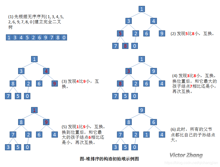
-
此时,整个序列的最大值就是堆顶的根节点
-
将其与末尾元素进行交换,此时末尾就为最大值
-
然后将剩余
n-1个元素重新构造成一个堆,这样就会得到n个元素的次小值。如此反复执行,便得到一个有序序列了
-
-
代码
1 2 3 4 5 6 7 8 9 10 11 12 13 14 15 16 17 18 19 20 21 22 23 24 25 26 27 28 29 30 31 32 33 34 35 36 37 38 39 40 41 42 43 44 45 46 47 48 49 50 51 52 53 54 55 56 57 58 59 60 61 62 63 64 65 66 67 68 69 70package sort; import java.util.Arrays; /* * 堆排序:升序排列 * */ public class heapSort { public static void main(String[] args) { int[] arr = {4, 13, 11, 0, 1, 2, 3, 4, 3, 2, 1, 6, 8, 5, 9, 14, 12, 9, 0}; System.out.println(Arrays.toString(sortArray(arr))); } //堆排序 public static int[] sortArray(int[] nums) { //建立初始大根堆 buildMaxHeap(nums); //调整大根堆 for (int i = nums.length - 1; i > 0; i--) { //将大根堆顶与最后一个元素交换,通过不断交换,最后得到一个升序数组(每次交换从堆中移出已排好序的元素,堆逐渐变小) swap(nums, 0, i); //调整剩余数组,使其满足大顶堆 maxHeapify(nums, 0, i); } return nums; } //建立初始大根堆 public static void buildMaxHeap(int[] nums) { //最后一个非叶子节点开始,这样不断地从左至右,从下至上的调整,每次调整只是调整最多三个节点的小堆,方便处理 for (int i = nums.length / 2 - 1; i >= 0; i--) { //调整每一个子树为大根堆 maxHeapify(nums, i, nums.length); } } //调整大根堆,第二个参数为堆顶,第三个参数为,堆的大小 public static void maxHeapify(int[] nums, int i, int heapSize) { //左子树 int l = 2 * i + 1; //右子树 int r = l + 1; //记录根结点、左子树结点、右子树结点三者中的最大值下标 int largest = i; //与左子树结点比较 if (l < heapSize && nums[l] > nums[largest]) { largest = l; } //与右子树结点比较 if (r < heapSize && nums[r] > nums[largest]) { largest = r; } //如果当前节点的左子树或右子树比它大,则赋值 if (largest != i) { //将最大值交换为根结点 swap(nums, i, largest); //再次调整交换数字后的大顶堆 //当树的深度够大时,如果没有下面这条语句, //也就是说,每次交换只会停留在每一个小堆(最多三个节点构成的小堆) //还需要递归看看其左右子树是否存在比当前节点大的数,有则交换上来,无则退出递归 maxHeapify(nums, largest, heapSize); } } //交换 public static void swap(int[] nums, int i, int j) { int temp = nums[i]; nums[i] = nums[j]; nums[j] = temp; } }
六、查找算法
查找是在大量的信息中寻找一个特定的信息元素,在计算机应用中,查找是常用的基本运算,例如编译程序中符号表的查找。本文简单概括性的介绍了常见的七种查找算法,说是七种,其实二分查找、插值查找以及斐波那契查找都可以归为一类——插值查找。插值查找和斐波那契查找是在二分查找的基础上的优化查找算法。
查找算法分类:
-
静态查找和动态查找;
注:静态或者动态都是针对查找表而言的。动态表指查找表中有删除和插入操作的表。
-
无序查找和有序查找。
无序查找:被查找数列有序无序均可,如顺序查找
有序查找:被查找数列必须为有序数列,如:二分查找,插值查找,斐波那契查找
二分查找,插值查找,斐波那契查找的原理类似,只是分割点的原理不同,二分查找是无脑二分,插值查找是自适应地趋向目标值(采用拉格朗日插值法),斐波那契查找分割是玄学黄金分割。
平均查找长度(Average Search Length,ASL):需和指定key进行比较的关键字的个数的期望值,称为查找算法在查找成功时的平均查找长度
对于含有n个数据元素的查找表,查找成功的平均查找长度为:ASL = Pi*Ci的和
Pi:查找表中第i个数据元素的概率
Ci:找到第i个数据元素时已经比较过的次数
1. 顺序查找
-
原理
说明:顺序查找适合于存储结构为顺序存储或链接存储的线性表。
基本思想:顺序查找也称为线性查找,属于无序查找算法。从数据结构线性表的一端开始,顺序扫描,依次将扫描到的结点关键字与给定值
k相比较,若相等则表示查找成功;若扫描结束仍没有找到关键字等于k的结点,表示查找失败。复杂度分析:
查找成功时的平均查找长度为:(假设每个数据元素的概率相等)
ASL = 1/n(1+2+3+…+n) = (n+1)/2;当查找不成功时,需要
n+1次比较,时间复杂度为O(n);所以,顺序查找的时间复杂度为O(n)。 -
代码实现
1 2 3 4 5 6 7 8 9 10 11 12 13 14 15 16 17 18 19package search; public class seqSearch { public static void main(String[] args) { int[] arr = {1, 4, -1, 2, -4, 8, 90}; int index = seqSearch(arr, 90); System.out.println("查找的元素在索引为" + index + "的位置"); } public static int seqSearch(int[] arr, int value) { for (int i = 0; i < arr.length; i++) { if (arr[i] == value) { return i; } } System.out.println("没有该数据"); return 0; } }
2. 二分查找
二分查找如下(本处文字用于本文锚点跳转,请勿删除)
-
原理
说明:元素必须是有序的,如果是无序的则要先进行排序操作。
**基本思想:**也称为是折半查找,属于有序查找算法。用给定值k先与中间结点的关键字比较,中间结点把线形表分成两个子表,若相等则查找成功;若不相等,再根据k与该中间结点关键字的比较结果确定下一步查找哪个子表,这样递归进行,直到查找到或查找结束发现表中没有这样的结点。
复杂度分析:最坏情况下,关键词比较次数为
log2(n+1),且期望时间复杂度为O(log2n);注:折半查找的前提条件是需要有序表顺序存储,对于静态查找表,一次排序后不再变化,折半查找能得到不错的效率。但对于需要频繁执行插入或删除操作的数据集来说,维护有序的排序会带来不小的工作量,那就不建议使用
-
代码实现
1 2 3 4 5 6 7 8 9 10 11 12 13 14 15 16 17 18 19 20 21 22 23 24 25 26 27 28 29 30 31 32 33 34 35 36 37 38 39 40 41 42 43 44 45 46 47package search; /* * 二分查找有序序列 * */ public class binarySearch { public static void main(String[] args) { int[] arr = {1, 2, 3, 5, 6, 10, 11}; int index = binarySearch1(arr,5); System.out.println("查找的元素在索引为" + index + "的位置"); int index1 = binarySearch2(arr, 4, 0, arr.length - 1); System.out.println("查找的元素在索引为" + index1 + "的位置"); } //折半查找:数组已经有序,从小到大的顺序 public static int binarySearch1(int[] arr, int value) { int left = 0, right = arr.length - 1; int mid = 0; while (left <= right) { mid = (left + right) / 2;//边界条件的移动也促使mid的移动 if (arr[mid] > value) {//value在arr[mid]之前 right = mid - 1;//将边界条件缩小至mid-1 } else if (arr[mid] < value) {//value在arr[mid]之后 left = mid + 1;//将边界条件扩大至mid+1 } else { return mid; } } System.out.println("数据不存在"); return -1; } //递归查找 public static int binarySearch2(int[] arr, int value, int left, int right) { int mid = left + (right - left) / 2;//避免数据过大 if (left > right) { System.out.println("数据不存在"); return -1; } if (arr[mid] < value) {//向右子序列递归 return binarySearch2(arr, value, mid + 1, right); } else if (arr[mid] > value) {//向左子序列递归 return binarySearch2(arr, value, left, mid - 1); } else {//递归结束条件 return mid; } } }
3. 插值查找
-
原理
在介绍插值查找之前,首先考虑一个新问题,为什么上述算法一定要是折半,而不是折四分之一或者折更多呢?打个比方,在英文字典里面查“apple”,你下意识翻开字典是翻前面的书页还是后面的书页呢?如果再让你查“zoo”,你又怎么查?很显然,这里你绝对不会是从中间开始查起,而是有一定目的的往前或往后翻。同样的,比如要在取值范围1 ~ 10000 之间 100 个元素从小到大均匀分布的数组中查找5, 我们自然会考虑从数组下标较小的开始查找。
经过以上分析,折半查找这种查找方式,不是自适应的(也就是说是傻瓜式的)。二分查找中查找点计算如下:
mid=(low+high)/2, 即mid=low+1/2*(high-low)通过类比,我们可以将查找的点改进为如下:
mid=low+(key-a[low])/(a[high]-a[low])*(high-low)也就是将上述的比例参数
1/2改进为自适应的,根据关键字在整个有序表中所处的位置,让mid值的变化更靠近关键字key,这样也就间接地减少了比较次数。**基本思想:**基于二分查找算法,将查找点的选择改进为自适应选择,可以提高查找效率。当然,差值查找也属于有序查找。
注:对于表长较大,而关键字分布又比较均匀的查找表来说,插值查找算法的平均性能比折半查找要好的多。反之,数组中如果分布非常不均匀,那么插值查找未必是很合适的选择。
复杂度分析:查找成功或者失败的时间复杂度均为
O(log2(log2n)) -
代码实现
1 2 3 4 5 6 7 8 9 10 11 12 13 14 15 16 17 18 19 20 21 22 23 24 25 26 27 28package search; /* * 插值查找,改进版二分查找,使用自适应的mid来靠近value,以避免盲目的分区,节省比较次数 * */ public class insertionSearch { public static void main(String[] args) { int[] arr = {1, 2, 3, 5, 6, 10, 11}; int index1 = insertionSearch(arr, 3, 0, arr.length - 1); System.out.println("查找的元素在索引为" + index1 + "的位置"); } public static int insertionSearch(int[] arr, int value, int left, int right) { // int mid = left + (right - left) / 2;//避免数据过大 int mid = left + (value - arr[left]) / (arr[right] - arr[left]) * (right - left);//自适应mid if (left > right) { System.out.println("数据不存在"); return -1; } if (arr[mid] < value) {//向右子序列递归 return insertionSearch(arr, value, mid + 1, right); } else if (arr[mid] > value) {//向左子序列递归 return insertionSearch(arr, value, left, mid - 1); } else {//递归结束条件 return mid; } } }
4. 斐波那契查找
-
原理
**基本思想:**斐波那契查找原理与前两种相似,仅仅改变了中间结点(mid)的位置,
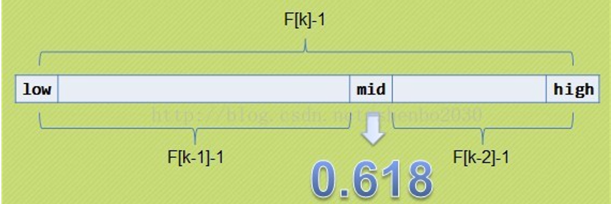
mid不再是中间或插值得到,而是位于黄金分割点附近,即mid=low+F(k-1)-1(F代表斐波那契数列)对
F(k-1)-1的理解: 由斐波那契数列F[k]=F[k-1]+F[k-2]的性质,可以得到(F[k]-1)=(F[k-1]-1)+(F[k-2]-1)+1。该式说明:只要顺序表的长度为F[k]-1,则可以将该表分成长度为F[k-1]-1和F[k-2]-1的两段,即如上图所示。从而中间位置为mid=low+F(k-1)-1。类似的,每一子段也可以用相同的方式分割。但顺序表长度n不一定刚好等于F[k]-1,所以需要将原来的顺序表长度n增加至F[k]-1。这里的k值只要能使得F[k]-1恰好大于或等于n即可,由以下代码得到,顺序表长度增加后,新增的位置(从n+1到F[k]-1位置),都赋为n位置的值即可。1while(n>fib(k)-1) k++;开始将k值与第
F(k-1)位置的记录进行比较(及mid=low+F(k-1)-1),比较结果也分为三种-
相等,
mid位置的元素即为所求。注意扩容后的数组长度带来的影响 -
大于,
low=mid+1,k-=2说明:
low=mid+1说明待查找的元素在[mid+1,high]范围内,k-=2说明范围[mid+1,high]内的元素个数为n-(F(k-1))= F(k)-1-F(k-1)=F(k)-F(k-1)-1=F(k-2)-1个,所以可以递归地应用斐波那契查找 -
小于,
high=mid-1,k-=1说明:
low=mid+1说明待查找的元素在[low,mid-1]范围内,k-=1说明范围[low,mid-1]内的元素个数为F(k-1)-1个,所以可以递归地应用斐波那契查找。
复杂度分析:最坏情况下,时间复杂度为
O(log2n),且其期望复杂度也为O(log2n)。 -
-
代码实现
1 2 3 4 5 6 7 8 9 10 11 12 13 14 15 16 17 18 19 20 21 22 23 24 25 26 27 28 29 30 31 32 33 34 35 36 37 38 39 40 41 42 43 44 45 46 47 48 49 50 51 52 53 54 55 56 57 58 59 60 61 62 63 64 65 66 67 68 69 70 71 72 73 74 75 76 77package search; import java.util.Arrays; /* * 斐波那契查找 * */ public class fibonacciSearch { public static int maxSize = 20; public static void main(String[] args) { int[] arr = {1, 8, 10, 89, 1000, 1234}; int index = fibonacciSearch(arr, 1000); System.out.println(index); } //斐波那契查找算法 public static int fibonacciSearch(int[] arr, int val) { int low = 0; int high = arr.length - 1;//代表原数组最高的下标4 int k = 0;//斐波那契分割数值的下标 int mid; int[] f = getFib(); //获取到斐波那契分割数值的下标 1 1 2 3 5 8 while (arr.length > f[k] - 1) {//6 2 k++;//4 } //因为f[k]值可能大于a的长度,因此我们需要使用Arrays类,构造一个新的数组,并指向a[] int[] temp = Arrays.copyOf(arr, f[k]); //填充新的数组,因为新数组长度如果比原数组大,多的部分会被填充0,因此需要使用最后面的最大值来填充,防止数组顺序被破坏 for (int i = high + 1; i < temp.length; i++) { temp[i] = arr[high]; } //找到中间值mid后开始查找 while (low <= high) {//只要这个条件满足,就可以继续查找 mid = low + f[k - 1] - 1;// if (val < temp[mid]) {//向左查找 high = mid - 1; //为什么是k-- //说明 //1.全部元素 = 前面的元素 + 后边元素 //2.f[k] = f[k-1]+f[k-2] //因为前面有f[k-1]个元素,所以可以继续拆分f[k-1] = f[k-2] + f[k-3] //即在f[k-1]的前面继续查找k-- //即下次循环mid = f[k-1-1]-1 k--; } else if (val > temp[mid]) { low = mid + 1; //为什么是k-=2 //说明 //继续拆分f[k-2] = f[k-3] + f[k-4] //即在f[k-2]的前面继续查找k-=2 //即下次循环mid = f[k-1-1-1]-1 k -= 2; } else { if (mid <= high) { return mid; } else { //数组扩容过,此时返回mid就会超出原数组的长度 return high; } } } return -1; } //生成一个斐波那契数列 public static int[] getFib() { int[] f = new int[maxSize]; f[0] = 0; f[1] = 1; for (int i = 2; i < maxSize; i++) { f[i] = f[i - 1] + f[i - 2]; } return f; } }
5. 哈希表数据结构
-
原理
散列表(Hash table,也叫哈希表),是根据关键码值(Key value)而直接进行访问的数据结构。也就是说,它通过把关键码值映射到表中一个位置来访问记录,以加快查找的速度。这个映射函数叫做散列函数,存放记录的数组叫做散列表。
可以使用数组+链表实现,或者使用数组+二叉数/二叉排序树实现(性能更高)。在业务里的应用可以是:使用哈希表构建自己项目的缓存中间层放在数据库和服务器之间(造个轮子)
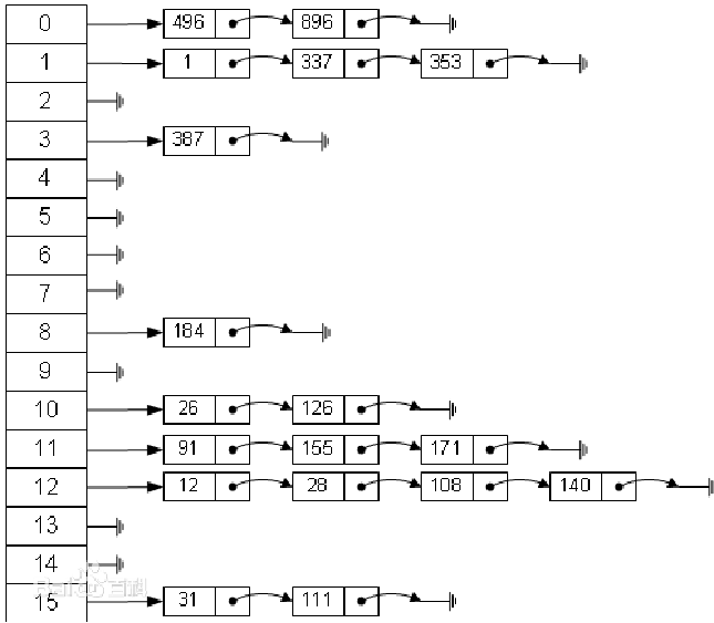
-
哈希表业务应用
题目:
有一个公司,当有新的员工来报道时,要求将该员工的信息加入 (id,性别,年龄,名字,住址..),当输入该员工的id时,要求查找到该员工的 所有信息. 要求: 不使用数据库,,速度越快越好=>哈希表(散列)、添加时,保证按照id从低到高插入
代码实现:
1 2 3 4 5 6 7 8 9 10 11 12 13 14 15 16 17 18 19 20 21 22 23 24 25 26 27 28 29 30 31 32 33 34 35 36 37 38 39 40 41 42 43 44 45 46 47 48 49 50 51 52 53 54 55 56 57 58 59 60 61 62 63 64 65 66 67 68 69 70 71 72 73 74 75 76 77 78 79 80 81 82 83 84 85 86 87 88 89 90 91 92 93 94 95 96 97 98 99 100 101 102 103 104 105 106 107 108 109 110 111 112 113 114 115 116 117 118 119 120 121 122 123 124 125 126 127 128 129 130 131 132 133 134 135 136 137 138 139 140 141 142 143 144 145 146 147 148 149 150 151 152 153 154 155 156 157 158 159 160 161 162 163 164 165 166 167 168 169 170 171 172 173 174 175 176 177 178 179 180 181 182 183 184 185 186 187 188 189 190 191 192 193 194 195 196 197 198 199 200 201 202 203 204 205 206 207 208 209 210 211 212 213 214 215 216 217 218 219 220 221 222 223 224 225package hashTable; /* * 哈希表 * */ public class hashTable { public static void main(String[] args) { hashTableManager hashTableManager = new hashTableManager(10); hashTableManager.add(new node(114, "cold bin", "重庆")); hashTableManager.add(new node(224, "wtl", "重庆")); hashTableManager.add(new node(334, "sss", "ss")); hashTableManager.add(new node(3, "bwj", "重庆")); hashTableManager.show(); hashTableManager.delete(224); hashTableManager.show(); hashTableManager.update(new node(334, "aaa", "")); hashTableManager.show(); node node = hashTableManager.findNode(224); if (node != null) { System.out.println("找到节点" + node); } } } class hashTableManager { int size;//哈希表的数组长度 nodeManager[] hashTable;//哈希表的内存结构 public hashTableManager(int size) { this.size = size; hashTable = new nodeManager[size]; //实例化数组里的对象 for (int i = 0; i < size; i++) { nodeManager nodeManager = new nodeManager(20); hashTable[i] = nodeManager; } } //散列函数 public int hashFunc(int id) { return id % this.size; } //添加 public void add(node node) { int nodeManagerNo = hashFunc(node.id); this.hashTable[nodeManagerNo].add(node); } public void delete(int id) { int nodeManagerNo = hashFunc(id); this.hashTable[nodeManagerNo].delete(id); } public void update(node node) { int nodeManagerNo = hashFunc(node.id); this.hashTable[nodeManagerNo].update(node); } //查询id对应的员工信息 public node findNode(int id) { int nodeManagerNo = hashFunc(id); return this.hashTable[nodeManagerNo].findNode(id); } //遍历 public void show() { for (int i = 0; i < this.size; i++) { if (!this.hashTable[i].isEmpty()) { System.out.print("哈希表第" + (i + 1) + "行:"); this.hashTable[i].show(); } else { System.out.println("哈希表第" + (i + 1) + "行为空"); } } } } class nodeManager { int maxSize;//节点最大容量 node head;//带数据的头节点 //初始化空的带头节点链表 public nodeManager(int maxSize) { this.head = new node(-1); this.maxSize = maxSize; } public boolean isEmpty() { return head.next == null; } public boolean isFull() { int num = 0; node temp = head; while (temp.next != null) { num++; temp = temp.next; } return num == maxSize - 1; } //增:按照id递增插入 public void add(node node) { if (isFull()) { System.out.println("链表已满"); return; } node temp = head; while (temp != null) { node beforeNode = temp; if (temp.next == null) { temp.next = node; return; } temp = temp.next; if (temp.id > node.id) { //记录对应编号节点的前一个节点位置,将新节点插入这个位置,意即beforeNode之后,temp之前; beforeNode.next = node; node.next = temp; System.out.println("插入成功"); return; } } System.out.println("没有找到编号"); } //删 public void delete(int id) { if (isEmpty()) { System.out.println("链表已空"); return; } node temp = head.next; while (temp != null) { node preNode = temp; temp = temp.next; if (temp.id == id) { preNode.next = temp.next; System.out.println("删除成功"); return; } } System.out.println("删除失败,没有该id"); } //改 public void update(node node) { if (isEmpty()) { System.out.println("链表已空"); return; } node temp = head.next; while (temp != null) { temp = temp.next; if (temp.id == node.id) { temp.name = node.name; temp.address = node.address; System.out.println("更新成功"); return; } } System.out.println("更新失败,没有该id"); } //查找节点 public node findNode(int id) { if (isEmpty()) { System.out.println("链表为空"); return null; } node temp = head; while (temp != null && temp.id != id) { temp = temp.next; } if (temp != null) { return temp; } else { System.out.println("没有该id"); return null; } } //查 public void show() { if (isEmpty()) { System.out.println("链表为空"); return; } node temp = head.next; System.out.print("链表:"); while (temp != null) { System.out.print(temp); temp = temp.next; } System.out.println(); } } class node { int id; String name; String address; node next; public node(int id, String name, String address) { this.id = id; this.name = name; this.address = address; } public node(int id) { this.id = id; } @Override public String toString() { return "node{" + "id=" + id + ", name='" + name + '\'' + ", address='" + address + '\'' + '}'; } }
七、树
为什么需要树这种数据结构
-
数组存储方式的分析
- 优点:通过下标方式访问元素,速度快。对于有序数组,还可使用二分查找提高检索速度
- 缺点:如果要检索具体某个值,或者插入值(按一定顺序)会整体移动,效率较低
-
链式存储方式的分析
- 优点:在一定程度上对数组存储方式有优化(比如:插入一个数值节点,只需要将插入节点,链接到链表中即可, 删除效率也很好)。
- 缺点:在进行检索时,效率仍然较低,比如(检索某个值,需要从头节点开始遍历)
-
树存储方式的分析
-
优点:能提高数据存储,读取的效率, 比如利用 二叉排序树(Binary Sort Tree),既可以保证数据的检索速度,同时也可以保证数据的插入,删除,修改的速度。案例:
[7, 3, 10, 1, 5, 9, 12]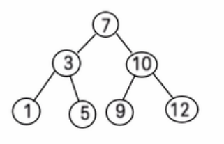
-
1. 二叉树
① 二叉树概念
下图有些错误:H、E、F、G才是叶子节点
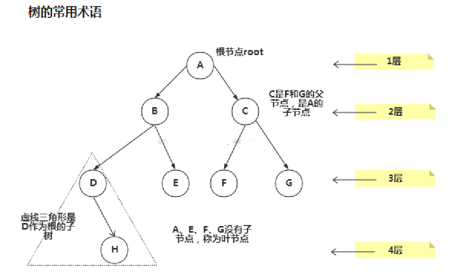
树的常用术语
- 节点
- 根节点
- 父节点
- 子节点
- 叶子节点 (没有子节点的节点)
- 节点的权(节点值)
- 路径(从root节点找到该节点的路线)
- 层
- 子树
- 树的高度(最大层数)
- 森林 :多颗子树构成森林
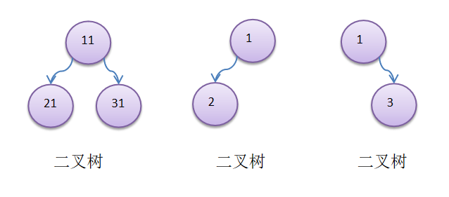
概念
-
树有很多种,每个节点最多只能有两个子节点的一种形式称为二叉树。二叉树的子节点分为左节点和右节点。
-
如果该二叉树的所有叶子节点都在最后一层,并且结点总数=
2^n -1(等比数列前n项和) ,n为层数,则我们称为满二叉树。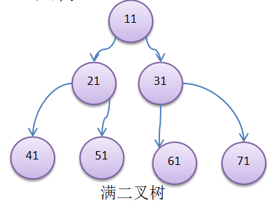
-
完全二叉树是由满二叉树而引出来的,若设二叉树的
深度为h,除第 h 层外,其它各层 (1~h-1) 的结点数都达到最大个数(即1~h-1层为一个满二叉树),第 h 层所有的结点都连续集中在最左边,这就是完全二叉树。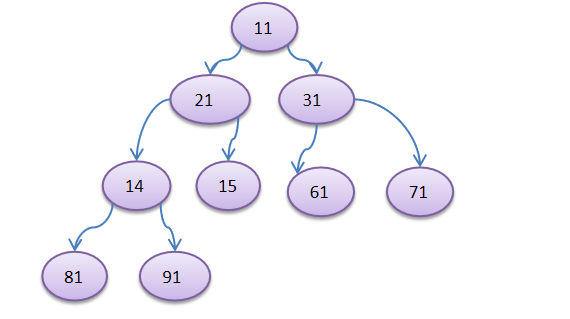
注意:完全二叉树 , 如果把 (61)节点删除,就不是完全二叉树了,因为叶子节点不连续了
② 二叉树遍历
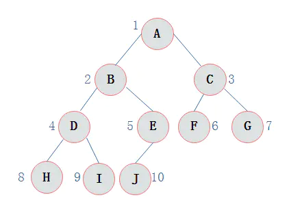
tips: 看输出父节点的顺序,就确定是前序,中序还是后序
示例一
-
节点
1 2 3 4 5 6 7 8 9 10 11 12 13 14 15 16 17 18 19 20 21 22 23class treeNode { int no; String name; treeNode leftChildNode; treeNode rightChildNode; public treeNode(int no, String name) { this.no = no; this.name = name; } @Override public String toString() { return "treeNode{" + "no=" + no + ", name='" + name + '\'' + '}'; } //前序遍历public void preShow() //中序遍历public void infixShow() //后序遍历public void postShow() } -
前序遍历: 先输出父节点,再假递归遍历左子树和右子树
前序就是 父节点->左子树->右子树
ABDHIEJCFG
1 2 3 4 5 6 7 8 9public void preShow(){ System.out.println(this); if (this.leftChildNode!=null){ this.leftChildNode.preShow();//此处还不叫递归,只是调用另一个对象的这个方法 } if (this.rightChildNode!=null){ this.rightChildNode.preShow(); } } -
中序遍历: 先假递归遍历左子树,再输出父节点,再假递归遍历右子树
中序就是左子树->父节点->右子树
则图所示二叉树的前序遍历输出为: HDIBJEAFCG
1 2 3 4 5 6 7 8 9public void infixShow(){ if (this.leftChildNode!=null){ this.leftChildNode.infixShow(); } System.out.println(this); if (this.rightChildNode!=null){ this.rightChildNode.infixShow(); } } -
后序遍历: 先递归遍历左子树,再递归遍历右子树,最后输出父节点
后序是 左子树 -> 右子树 ->父节点
HIDJEBFGCA
1 2 3 4 5 6 7 8 9public void postShow(){ if (this.leftChildNode!=null){ this.leftChildNode.postShow(); } if (this.rightChildNode!=null){ this.rightChildNode.postShow(); } System.out.println(this); }
示例二
-
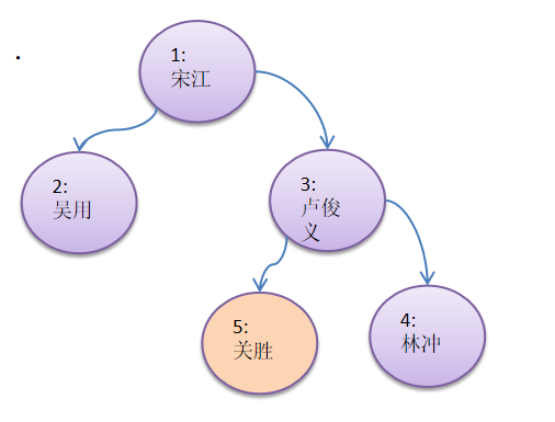
前上图的 3号节点 “卢俊” , 增加一个左子节点 [5, 关胜]
代码实现
1 2 3 4 5 6 7 8 9 10 11 12 13 14 15 16 17 18 19 20 21 22 23 24 25 26 27 28 29 30 31 32 33 34 35 36 37 38 39 40 41 42 43 44 45 46 47 48 49 50 51 52 53 54 55 56 57 58 59 60 61 62 63 64 65 66 67 68 69 70 71 72 73 74 75 76 77 78 79 80 81 82 83 84 85 86 87 88 89 90 91 92 93 94 95 96 97 98 99 100 101 102 103 104 105 106 107 108 109 110 111 112 113 114 115 116 117 118 119 120 121 122 123 124 125 126 127 128 129 130 131 132 133 134 135 136 137 138 139 140 141 142 143 144 145 146 147package binaryTree; public class binaryTree { public static void main(String[] args) { treeManager treeManager = new treeManager(new treeNode(1, "宋江")); treeNode n2 = new treeNode(2, "吴用"); treeNode n3 = new treeNode(3, "卢俊义"); treeNode n4 = new treeNode(4, "林冲"); treeManager.root.leftChildNode = n2; treeManager.root.rightChildNode = n3; n3.rightChildNode = n4; System.out.println("前序遍历:"); treeManager.preShow(); System.out.println(); System.out.println("后序遍历:"); treeManager.postShow(); System.out.println(); System.out.println("中序遍历:"); treeManager.infixShow(); System.out.println("插入节点后"); treeNode n5 = new treeNode(5, "关胜"); treeManager.add(n5); System.out.println("前序遍历:"); treeManager.preShow(); System.out.println(); System.out.println("后序遍历:"); treeManager.postShow(); System.out.println(); System.out.println("中序遍历:"); treeManager.infixShow(); } } class treeManager { treeNode root; public treeManager(treeNode root) { this.root = root; } //添加节点 public void add(treeNode node) { root.add(node); } public boolean isEmpty() { return this.root == null; } public void preShow() { if (isEmpty()) { System.out.println("树为空"); return; } root.preShow(); } public void infixShow() { if (isEmpty()) { System.out.println("树为空"); return; } root.infixShow(); } public void postShow() { if (isEmpty()) { System.out.println("树为空"); return; } root.postShow(); } } class treeNode { int no; String name; treeNode leftChildNode; treeNode rightChildNode; public treeNode(int no, String name) { this.no = no; this.name = name; } @Override public String toString() { return "treeNode{" + "no=" + no + ", name='" + name + '\'' + '}'; } //前序遍历 public void add(treeNode node) { if (this.no == 3) { this.leftChildNode = node; } if (this.leftChildNode != null) { this.leftChildNode.add(node); } if (this.rightChildNode != null) { this.rightChildNode.add(node); } } public void preShow() { System.out.println(this); if (this.leftChildNode != null) { this.leftChildNode.preShow(); } if (this.rightChildNode != null) { this.rightChildNode.preShow(); } } //中序遍历 public void infixShow() { if (this.leftChildNode != null) { this.leftChildNode.infixShow(); } System.out.println(this); if (this.rightChildNode != null) { this.rightChildNode.infixShow(); } } //后序遍历 public void postShow() { if (this.leftChildNode != null) { this.leftChildNode.postShow(); } if (this.rightChildNode != null) { this.rightChildNode.postShow(); } System.out.println(this); } } -
使用前序,中序,后序遍历,请写出各自输出的顺序是什么
1 2 3前序遍历:父节点->左子树->右子树 1 2 3 5 4 中序遍历:左子树->父节点->右子树 2 1 5 3 4 后序遍历:左子树 -> 右子树 ->父节点 2 5 4 3 1
③ 二叉树查找
-
前序查找
1 2 3 4 5 6 7 8 9 10 11 12 13 14 15 16 17 18 19 20 21public treeNode preSearch(int no) { System.out.println("进入前序查找"); //如果当前节点满足,则返回当前节点 if (this.no == no) { return this; } treeNode node = null; //再向左子树递归 if (this.leftChildNode != null) { node = this.leftChildNode.preSearch(no); } //先校验左子树递归结果,不然会被右子树的结果给覆盖掉 if (node != null) { return node; } //再向右子树递归 if (this.rightChildNode != null) { node = this.rightChildNode.preSearch(no); } return node; } -
中序查找
1 2 3 4 5 6 7 8 9 10 11 12 13 14 15 16 17 18 19 20public treeNode infixSearch(int no) { treeNode node = null; if (this.leftChildNode != null) { node = this.leftChildNode.infixSearch(no); } //如果已找到提前返回 if (node != null) { return node; } System.out.println("进入中序查找"); if (this.no == no) { return this; } if (this.rightChildNode != null) { node = this.rightChildNode.infixSearch(no); } return node; } -
后序查找
1 2 3 4 5 6 7 8 9 10 11 12 13 14 15 16 17 18 19 20 21 22 23 24public treeNode postSearch(int no) { treeNode node = null; if (this.leftChildNode != null) { node = this.leftChildNode.postSearch(no); } //左子节点找到要返回,否则会被右子节点覆盖掉 if (node != null) { return node; } if (this.rightChildNode != null) { node = this.rightChildNode.postSearch(no); } //右子节点不为空,需要提前返回 if (node != null) { return node; } System.out.println("进入后续查找"); if (this.no == no) { return this; } return null; }
④ 二叉树删除
-
删除节点及其子树
1 2 3 4 5 6 7 8 9 10 11 12 13 14 15 16 17 18 19 20 21public boolean delete(int no) { boolean res = false; //左子节点不为空,且编号相同,删除该节点或其子树 if (this.leftChildNode != null && this.leftChildNode.no == no) { this.leftChildNode = null; return true; } //右子节点不为空,且编号相同,删除该节点或其子树 if (this.rightChildNode != null && this.rightChildNode.no == no) { this.rightChildNode = null; return true; } //如果没有找到,继续递归 if (this.leftChildNode != null) { res = this.leftChildNode.delete(no); } if (this.rightChildNode != null) { res = this.rightChildNode.delete(no); } return res; } -
只删除节点
规则:
-
如果要删除的节点是非叶子节点,现在我们不希望将该非叶子节点为根节点的子树删除,需要指定规则, 假如规定如下:
-
如果该非叶子节点A只有一个子节点B,则子节点B替代节点A
-
如果该非叶子节点A有左子节点B和右子节点C,则让左子节点B替代节点A
代码
1 2 3 4 5 6 7 8 9 10 11 12 13 14 15 16 17 18 19 20 21 22 23 24 25 26 27 28 29 30 31 32 33 34 35 36 37 38 39 40 41 42 43 44 45 46 47 48public boolean delete2(int no) { boolean res =false; if (this.leftChildNode!=null&&this.leftChildNode.no==no){ //判断删除节点是否含有子树 if (this.leftChildNode.leftChildNode==null&&this.leftChildNode.rightChildNode==null){ //无子树,删除当前节点 this.leftChildNode=null; } else if (this.leftChildNode.leftChildNode!=null&&this.leftChildNode.rightChildNode==null) { //有左子树,无右子树,左子树代替删除节点 this.leftChildNode=this.leftChildNode.leftChildNode; } else if (this.leftChildNode.leftChildNode == null && this.leftChildNode.rightChildNode != null) { //无左子树,有右子树,右子树代替删除节点 this.leftChildNode=this.leftChildNode.rightChildNode; }else { //左右子树都有,左子树节点代替删除节点 this.leftChildNode=this.leftChildNode.leftChildNode; } return true; } if (this.rightChildNode!=null&&this.rightChildNode.no==no){ //判断删除节点是否含有子树 if (this.rightChildNode.leftChildNode==null&&this.rightChildNode.rightChildNode==null){ //无子树,删除当前节点 this.rightChildNode=null; } else if (this.rightChildNode.leftChildNode!=null&&this.rightChildNode.rightChildNode==null) { //有左子树,无右子树,左子树代替删除节点 this.rightChildNode=this.rightChildNode.leftChildNode; } else if (this.rightChildNode.leftChildNode == null && this.rightChildNode.rightChildNode != null) { //无左子树,有右子树,右子树代替删除节点 this.rightChildNode=this.rightChildNode.rightChildNode; }else { //左右子树都有,左子树节点代替删除节点 this.rightChildNode=this.rightChildNode.leftChildNode; } return true; } if (this.leftChildNode!=null){ res=this.leftChildNode.delete(no); } //提前返回结果,避免左子树覆盖 if (res){ return true; } if (this.rightChildNode!=null){ res=this.rightChildNode.delete(no); } return res; } -
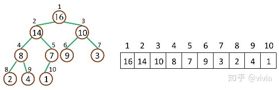
⑤ 顺序存储二叉树
(跳转的锚点)
从数据存储来看,数组存储方式和树的存储方式可以相互转换,即数组可以转换成树,树也可以转换成数组,看右面的示意图。也即,将数组通过某种关系可以看成一颗完全二叉树进行遍历,相应地一颗二叉树也可以通过某种关系看成数组进行遍历
概念:
- 顺序二叉树通常只考虑完全二叉树
- 第n个元素的左子节点为
2 * n + 1 - 第n个元素的右子节点为
2 * n + 2 - 第n个元素的父节点为
(n-1) / 2 - n : 表示二叉树中的第几个元素(按0开始编号如图所示)
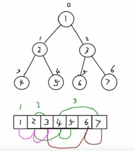
顺序存储二叉树的遍历:
|
|
⑥ 线索化二叉树
-
线索化概述:
对于一个二叉树来说,其二叉链表表示形式中正好有两个指针域,一个左子树指针域,一个右子树指针域。并且对于一个有
n个节点的二叉链表, 每个节点有指向左右孩子的两个指针域,所以共是2n个指针域。而n个节点的二叉树一共有n-1条分支数,也就是说,其实是存在2n-(n-1) = n+l个空指针域。将这些空指针利用起来,其中一个指针用作前驱指针,另一个指针指向后继指针,那么这样的话,这颗二叉树的遍历就不需要使用递归来进行,因为线索化的二叉树其实是一个双向链表(有序链表),也利用了那些空闲的空指针资源。前驱指针(节点):按照二叉树的某种序列遍历方式(前序、中序、后序等)得到的有序结果,某个节点的左子树为空就按这个遍历顺序指向当前节点的前一个结点,即前驱节点
后驱指针(节点):按照二叉树的某种序列遍历方式(前序、中序、后序等)得到的有序结果,某个节点的右子树为空就按这个遍历顺序指向当前节点的后一个结点,即后继节点
以上两个属性通过节点的
leftTag和rightTag区分 -
前序线索化
1 2 3 4 5 6 7 8 9 10 11 12 13 14 15public void preThreadOrder(treeNode1 node) { if (node == null) return; if (node.leftChildNode == null) { node.leftChildNode = this.preNode; node.leftTag = 1; } //右子树为空,指向后继节点:将前一个节点记录下来,当前节点node是preNode的后继节点,因此将后继节点指向preNode的空右子节点 if (this.preNode != null && this.preNode.rightChildNode == null) { this.preNode.rightChildNode = node; this.preNode.rightTag = 1; } this.preNode = node;//记录下一个节点 if (node.leftTag == 0) preThreadOrder(node.leftChildNode);//防止陷入无限循环 if (node.rightTag == 0) preThreadOrder(node.rightChildNode); } -
遍历前序线索化二叉树
由于二叉树已经线索化,原来的二叉树已经发生改变,不能再使用简单的前序遍历来遍历,采用新的方式(类似于遍历双向链表)
1 2 3 4 5 6 7 8 9 10 11 12 13 14 15 16 17 18 19 20public void preThreadList(treeNode1 root) { treeNode1 node = root; if (node == null) return; while (node != null) { //一直沿左子树遍历,直到遇到线索 while (node.leftTag == 0) { System.out.println(node); node = node.leftChildNode; } System.out.println(node); //此时已遍历一颗子树的根节点和左子树 //再遍历其后继节点 while (node.rightTag == 1) { node = node.rightChildNode; System.out.println(node); } //遇到当前节点无线索时,表示此时的节点有左右子树,左边已经遍历,该遍历右子树 node = node.rightChildNode; } } -
中序线索化
1 2 3 4 5 6 7 8 9 10 11 12 13 14 15 16 17 18 19 20public void infixThreadOrder(treeNode1 node) { //递归结束 if (node == null) return; //递归左子树 infixThreadOrder(node.leftChildNode); //将当前节点进行线索化 //当左子树为空,指向前驱节点 if (node.leftChildNode == null) { node.leftChildNode = this.preNode; node.leftTag = 1; } //右子树为空,指向后继节点:将前一个节点记录下来,当前节点node是preNode的后继节点,因此将后继节点指向preNode的空右子节点 if (this.preNode != null && this.preNode.rightChildNode == null) { this.preNode.rightChildNode = node; this.preNode.rightTag = 1; } this.preNode = node; //递归右子树 infixThreadOrder(node.rightChildNode); } -
遍历中序线索化二叉树
1 2 3 4 5 6 7 8 9 10 11 12 13 14 15 16public void infixThreadList(treeNode1 root) { treeNode1 node = root; while (node != null) { //找到遍历开始节点,中序遍历是最后一个左子节点 while (node.leftTag == 0) node = node.leftChildNode; //输出当前节点 System.out.println(node); //不断找寻后继节点 while (node.rightTag == 1) { node = node.rightChildNode;//获取后继节点 System.out.println(node); } //替换这个遍历的节点为前驱 node = node.rightChildNode; } } -
后序线索化
1 2 3 4 5 6 7 8 9 10 11 12 13 14 15 16public void postThreadOrder(treeNode1 node) { if (node == null) return; if (node.leftTag == 0) postThreadOrder(node.leftChildNode); if (node.rightTag == 0) postThreadOrder(node.rightChildNode); if (node.leftChildNode == null) { node.leftChildNode = this.preNode; node.leftTag = 1; } if (this.preNode != null && this.preNode.rightChildNode == null) { this.preNode.rightChildNode = node; this.preNode.rightTag = 1; } this.preNode = node; } -
遍历后序线索化二叉树
1 2 3 4 5 6 7 8 9 10 11 12 13 14 15 16 17 18 19 20 21 22 23 24 25 26 27 28 29 30public void postThreadList(treeNode1 root) { treeNode1 node = root; if (node == null) return; //遍历找到最左子节点,从此处开始遍历 while (node != null && node.leftTag == 0) node = node.leftChildNode; //暂存上一个节点 treeNode1 preNode = null; while (node != null) { //找到后序遍历输出的头节点时,不断输出后继节点 while (node.rightTag == 1) { System.out.println(node); preNode = node;//记录上一个遍历的节点 node = node.rightChildNode; } //如果上一个处理的节点当前节点的右子节点,则说明左右子树处理完毕,继续处理父节点 while (node.rightChildNode == preNode) { System.out.println(node); if (node.parentNode == null) return; preNode = node; node = node.parentNode;//需要记录父节点 } //如果上一个处理的节点是当前节点的左子节点 if (node.leftChildNode == preNode) { //找到右子树的最左子节点 node = node.rightChildNode; while (node != null && node.leftTag == 0) node = node.leftChildNode; } } } -
前序、中序、后序线索化比较
- 前序线索化二叉树遍历相对最容易理解,实现起来也比较简单。由于前序遍历的顺序是:根左右,所以从根节点开始,沿着左子树进行处理,当子节点的left指针类型是线索时,说明到了最左子节点,然后处理子节点的right指针指向的节点,可能是右子树,也可能是后继节点,无论是哪种类型继续按照上面的方式(先沿着左子树处理,找到子树的最左子节点,然后处理right指针指向),以此类推,直到节点的right指针为空,说明是最后一个,遍历完成。
- 中序线索化二叉树的网上相关介绍最多。中序遍历的顺序是:左根右,因此第一个节点一定是最左子节点,先找到最左子节点,依次沿着right指针指向进行处理(无论是指向子节点还是指向后继节点),直到节点的right指针为空,说明是最后一个,遍历完成。
- 后序遍历线索化二叉树最为复杂,通用的二叉树数节点存储结构不能够满足后序线索化,因此我们扩展了节点的数据结构,增加了父节点的指针。后序的遍历顺序是:左右根,先找到最左子节点,沿着right后继指针处理,当right不是后继指针时,并且上一个处理节点是当前节点的右节点,则处理当前节点的右子树,遍历终止条件是:当前节点是root节点,并且上一个处理的节点是root的right节点。
2. 树结构的实际应用
① 堆排序
如右:锚点连接
② 赫夫曼树
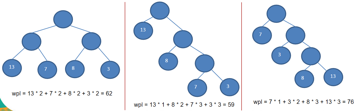
给定n个权值作为n个叶子结点,构造一棵二叉树,若该树的带权路径长度(wpl)达到最小,称这样的二叉树为最优二叉树,也称为哈夫曼树(Huffman Tree), 还有的书翻译为霍夫曼树。赫夫曼树是带权路径长度最短的树,权值较大的结点离根较近。
路径和路径的长度:在一棵树中,从一个结点往下可以达到的孩子或孙子结点之间的通路,称为路径。通路中分支节点的数目称为路径长度。若规定根结点的层数为1,则从根结点到第L层结点的路径长度为L-1
结点的权及带权路径长度:若将树中结点赋给一个有着某种含义的数值,则这个数值称为该结点的权。结点的带权路径长度为:从根结点到该结点之间的路径长度与该结点的权的乘积
树的带权路径长度:树的带权路径长度规定为所有叶子结点的带权路径长度之和,记为WPL(weighted path length) ,权值越大的结点离根结点越近的二叉树才是最优二叉树。WPL最小的就是赫夫曼树
构成赫夫曼树的步骤:
-
从小到大进行排序, 将每一个数据,每个数据都是一个节点,每个节点可以看成是一颗最简单的二叉树
-
取出根节点权值最小的两颗二叉树
-
组成一颗新的二叉树, 该新的二叉树的根节点的权值是前面两颗二叉树根节点权值的和
-
再将这颗新的二叉树,以根节点的权值大小 再次排序,不断重复1-2-3-4的步骤,直到数列中,所有的数据都被处理,就得到一颗赫夫曼树
1 2 3 4 5 6 7 8 9 10 11 12 13 14 15 16 17 18 19 20 21 22 23 24 25 26 27 28 29 30 31 32 33 34 35 36 37 38 39 40 41 42 43 44 45 46 47 48 49 50 51 52 53 54 55 56 57 58 59 60 61 62 63 64 65 66 67 68 69package binaryTree; import java.util.ArrayList; import java.util.Collections; /* * 赫夫曼树创建 * */ public class huffmanTree { public static void main(String[] args) { int[] arr = {13, 7, 8, 3, 29, 6, 1}; node tree = createHuffmanTree(arr); tree.preShow(tree); } public static node createHuffmanTree(int[] arr) { //创建节点,并塞入集合之中 ArrayList<node> nodes = new ArrayList<>(); for (int val : arr) { nodes.add(new node(val)); } while (nodes.size() > 1) { //排序 Collections.sort(nodes); //去除权值最小的两个node组成新的二叉树 node left = nodes.get(0); node right = nodes.get(1); node parent = new node(left.val + right.val); parent.left = left; parent.right = right; nodes.remove(0); nodes.remove(0);//这里的索引应该还是0,前面已经移除了一个元素 //将新的节点加进去 nodes.add(parent); } return nodes.get(0); } } class node implements Comparable<node> { int val;//哈夫曼树的权值 node left; node right; public node(int val) { this.val = val; } @Override public String toString() { return "node{" + "val=" + val + '}'; } @Override public int compareTo(node o) { return this.val - o.val; } public void preShow(node root) { node n = root; if (n == null) return; System.out.println(n); //左右子节点分别递归 if (n.left != null) preShow(n.left); if (n.right != null) preShow(n.right); } }
③ 赫夫曼编码
赫夫曼编码也翻译为哈夫曼编码(Huffman Coding),又称霍夫曼编码,是一种编码方式, 属于一种程序算法。赫夫曼编码是赫哈夫曼树在电讯通信中的经典的应用之一。赫夫曼编码广泛地用于数据文件压缩。其压缩率通常在20%~90%之间赫夫曼码是可变字长编码(VLC)的一种。Huffman于1952年提出一种编码方法,称之为最佳编码
-
变长编码(❌)
1 2 3 4i like like like java do you like a java// 共40个字符(包括空格) d:1 y:1 u:1 j:2 v:2 o:2 l:4 k:4 e:4 i:5 a:5 :9 // 各个字符对应的个数,9对应的是空格 0= , 1=a, 10=i, 11=e, 100=k, 101=l, 110=o, 111=v, 1000=j, 1001=u, 1010=y, 1011=d说明:按照各个字符出现的次数进行编码,原则是出现次数越多的,则编码越小,比如 空格出现了9次,编码为0,其它依次类推。按照上面给各个字符规定的编码,则我们在传输"i like like like java do you like a java"数据时,编码就是
10010110100...字符的编码都不能是其他字符编码的前缀,符合此要求的编码叫做前缀编码, 即不能匹配到重复的编码。意思是:当计算机在扫描编码数据时,首先得到
1,匹配a字符,但是后面还有个0,可以匹配空格,也可以10匹配i字符,这样的编码方式就导致某个字符对应的编码是另一个字符对应编码的前缀(即不符合前缀编码),这样就存在不好解码的问题 -
赫夫曼编码
-
赫夫曼编码原理
1 2 3 4i like like like java do you like a java // 共40个字符(包括空格) d:1 y:1 u:1 j:2 v:2 o:2 l:4 k:4 e:4 i:5 a:5 :9 各个字符对应的个数按照上面字符出现的次数构建一颗赫夫曼树, 次数作为权值(如图):
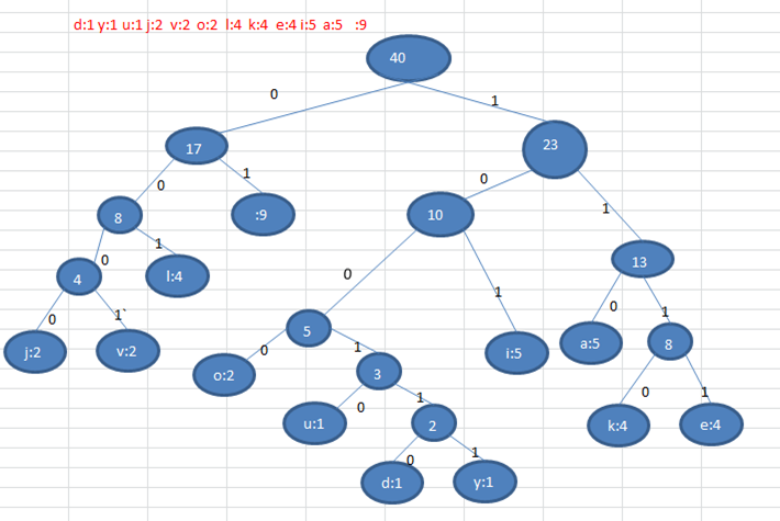
根据赫夫曼树,给各个字符规定编码,向左的路径为0,向右的路径为1。(一定是前缀编码)编码如下:
1o: 1000 u: 10010 d: 100110 y: 100111 i: 101a : 110 k: 1110 e: 1111 j: 0000 v: 0001l: 001 : 01//空格按照上面的赫夫曼编码,我们的
i like like like java do you like a java字符串对应的编码为 (注意这里我们使用的无损压缩):11010100110111101111010011011110111101001101111011110100001100001110011001111000011001111000100100100110111101111011100100001100001110长度为:133
说明:原来长度是359,压缩了
(359-133)/359 = 62.9%。此编码满足前缀编码, 即字符的编码都不能是其他字符编码的前缀,不会造成匹配的多义性注意:这个赫夫曼树根据排序方法不同,也可能不太一样,这样对应的赫夫曼编码也不完全一样,但是
wpl是一样的,都是最小的, 比如:如果我们让每次生成的新的二叉树总是排在权值相同的二叉树的最后一个,则生成的二叉树为:
-
最佳实践–数据压缩与解压
将给出的一段文本,比如 “i like like like java do you like a java” , 根据前面的讲的赫夫曼编码原理,对其进行数据压缩处理 ,形式如下
11010100110111101111010011011110111101001101111011110100001100001110011001111000011001111000100100100110111101111011100100001100001110步骤1:根据赫夫曼编码压缩数据的原理,需要创建 “i like like like java do you like a java” 对应的赫夫曼树
步骤2:生成赫夫曼树对应的赫夫曼编码表,如下表
1:=01 a=100 d=11000 u=11001 e=1110 v=11011 i=101 y=11010 j=0010 k=1111 l=000 o=0011步骤3:使用赫夫曼编码来生成赫夫曼编码数据 ,即按照上面的赫夫曼编码表,将"i like like like java do you like a java"字符串生成对应的编码数据, 形式如下(目前只是编码好了,还未压缩)
11010100010111111110010001011111111001000101111111100100101001101110001110000011011101000111100101000101111111100110001001010011011100步骤4:将编码好的数据进行压缩,每8位二进制字符串为组成一个十进制或16进制数据,这样可以减少二进制字符串的长度,从而达到压缩的目的,值得注意的是最后8位的特殊处理,因为可能赫夫曼编码过后不满足8位,此时就需要记录这个有多少位。
1 2 3 4 5 6 7 8 9 10 11 12 13 14 15 16 17 18 19 20 21 22 23 24 25 26 27 28 29 30 31 32 33 34 35 36 37 38 39 40 41 42 43 44 45 46 47 48 49 50 51 52 53 54 55 56 57 58 59 60 61 62 63 64 65 66 67 68 69 70 71 72 73 74 75 76 77 78 79 80 81 82 83 84 85 86 87 88 89 90 91 92 93 94 95 96 97 98 99 100 101 102 103 104 105 106 107 108 109 110 111 112 113 114 115 116 117 118 119 120 121 122 123 124 125 126 127 128 129 130 131 132 133 134 135 136 137 138 139 140 141 142 143 144 145 146 147 148 149 150 151 152 153 154 155 156 157 158 159 160 161 162 163 164 165 166 167 168 169 170 171 172 173 174 175 176 177 178 179 180 181 182 183 184 185 186 187 188 189 190 191 192 193 194 195 196 197 198 199 200 201 202 203 204 205 206 207 208 209 210 211 212 213 214 215 216 217 218 219 220 221 222 223 224 225 226 227 228package binaryTree; import java.util.*; public class huffmanCode { static Map<Byte, String> CodeTable = new HashMap<>();//哈夫曼编码表 static int LastLength = -1;//记录最后一个数压缩的长度,方便解压正确 public static void main(String[] args) { String text = "i like like like java do you like a java -asasda 1 0 -1"; System.out.println("字符串长度:" + text.length()); //转化为字符数组 byte[] chs = text.getBytes(); System.out.println(Arrays.toString(huffmanZip(chs))); System.out.println(new String(decode(CodeTable, huffmanZip(chs)))); } public static byte[] decode(Map<Byte, String> huffmanCodeTable, byte[] huffmanBytes) { //将压缩数据转化为二进制字符串,即解压 StringBuilder builder = new StringBuilder(); boolean flag = false; for (int i = 0; i < huffmanBytes.length; i++) { if (i == huffmanBytes.length - 1) flag = true; String bitString = bytesToBitString(flag, huffmanBytes[i]); builder.append(bitString); System.out.println("结果:" + huffmanBytes[i] + " " + bitString); } System.out.println(builder); //根据哈夫曼编码表,将二进制字符串还原成源字符串,即编码 //调换键值顺序 Map<String, Byte> map = new HashMap<>(); for (Map.Entry<Byte, String> entry : huffmanCodeTable.entrySet()) { map.put(entry.getValue(), entry.getKey()); } //集合存储byte List<Byte> list = new ArrayList<>(); for (int i = 0; i < builder.length(); ) { int count = 1;//计数指针 boolean f = true; Byte b = null; while (f) { String key = builder.substring(i, i + count); b = map.get(key); if (b == null) { count++; } else { f = false; } } list.add(b); i += count; } byte[] bytes = new byte[list.size()]; for (int i = 0; i < bytes.length; i++) { bytes[i] = list.get(i); } return bytes; } //将一个byte转化为有个二进制字符串,flag标志最后一位 public static String bytesToBitString(boolean flag, byte b) { StringBuilder prefix = new StringBuilder();//用于正数前缀补零 String str = Integer.toBinaryString(b); int len = str.length(); if (flag) {//如果是最后一位,可能会少于8位,前面记录在LastLength全局变量里 //如果是正数,需要补高位,补足LastLength位 if (b >= 0) { while (len < LastLength) { prefix.append('0'); len++; } return prefix + str; } else {//如果是负数,就需要只保留后8位 return str.substring(str.length() - 8); } } else {//不是最后一位,一定是满8位 //如果是正数,需要补高位补足8位 if (b >= 0) { while (len < 8) { prefix.append('0'); len++; } return prefix + str; } else {//如果是负数,就需要只保留后8位 return str.substring(str.length() - 8); } } } //将原始字符串的bytes数据编码并压缩,返回压缩结果 public static byte[] huffmanZip(byte[] bytes) { //根据原始数据生成哈夫曼编码树 List<node1> nodes = getNodes(bytes); node1 root = createHuffmanTree(nodes); //根据生成的哈夫曼编码树生成编码表 StringBuilder result = new StringBuilder(); getHuffmanCode(root, "", result); //根据哈夫曼编码表和原始bytes数组数据,进行压缩 return zip(bytes, CodeTable); } //根据赫夫曼编码表,将字符串的byte数组,返回一个赫夫曼编码,压缩后的byte数组 public static byte[] zip(byte[] oldBytes, Map<Byte, String> codeTable) { StringBuilder builder = new StringBuilder(); //根据哈夫曼编码表,将byte数组转化为编码数据(变长了) //这个编码数据还不是最后的压缩结果,根据显示,显然这个数据的长度还变长了,并没有压缩 for (byte b : oldBytes) { builder.append(codeTable.get(b)); } System.out.println(builder); //将编码的字符串数据进行压缩,每8位一个字节数据,不足8位的往前补一位 int len; int index = 0; if (builder.length() % 8 == 0) len = builder.length() / 8; else len = builder.length() / 8 + 1; //创建压缩后的byte数组 byte[] compressedBytes = new byte[len]; for (int i = 0; i < builder.length(); i += 8) { String strByte; if (i + 8 > builder.length()) {//将最后剩余的字节加进去(可能少于8个) strByte = builder.substring(i); //todo 为方便解码最后一位数字,需要记录最后一位byte数字的二进制长度 LastLength = strByte.length(); } else { strByte = builder.substring(i, i + 8); } //每8个二进制位压缩成一个数字: compressedBytes[index++] = (byte) Integer.parseInt(strByte, 2); } return compressedBytes; } //得到所有叶子节点的哈夫曼编码表 public static void getHuffmanCode(node1 node, String code, StringBuilder result) { StringBuilder code1 = new StringBuilder(result); code1.append(code); if (node != null) { if (node.data == 0) {//非叶子节点 getHuffmanCode(node.left, "0", code1);//左子节点递归 getHuffmanCode(node.right, "1", code1);//右子节点递归 } else {//叶子节点 CodeTable.put(node.data, code1.toString()); } } } //创建哈夫曼树,返回父节点 public static node1 createHuffmanTree(List<node1> nodes) { while (nodes.size() > 1) { //排序 Collections.sort(nodes); //取出首两个节点 node1 left = nodes.get(0); node1 right = nodes.get(1); node1 parent = new node1(left.weight + right.weight); //组成二叉树 parent.left = left; parent.right = right; //移除首两个节点 nodes.remove(0); nodes.remove(0); nodes.add(parent); } return nodes.get(0); } //统计每个字符出现的次数(权重),然后记录在链表里 public static List<node1> getNodes(byte[] chs) { ArrayList<node1> nodes = new ArrayList<>(); HashMap<Byte, Integer> map = new HashMap<>(); for (byte ch : chs) { Integer weight = map.get(ch); if (weight == null) { map.put(ch, 1); } else { map.put(ch, weight + 1); } } //将map里的值转化为node1并化为链表 //遍历map for (Map.Entry<Byte, Integer> entry : map.entrySet()) { nodes.add(new node1(entry.getKey(), entry.getValue())); } return nodes; } } class node1 implements Comparable<node1> { byte data;//存放的数据 int weight;//权值 node1 left; node1 right; //前序遍历 public void preShow(node1 root) { node1 temp = root; if (temp == null) return; System.out.println(temp); if (temp.left != null) preShow(temp.left); if (temp.right != null) preShow(temp.right); } @Override public String toString() { //为空的权值不输出 if (data == 0) return "node1{weight=" + weight + '}'; return "node1{" + "data=" + data + ", weight=" + weight + '}'; } public node1(int weight) { this.weight = weight; } public node1(byte data, int weight) { this.data = data; this.weight = weight; } @Override public int compareTo(node1 o) { return this.weight - o.weight; } }
-
④ 二叉排序树或搜索树(BST)
-
与数组、链表比较分析
数组:未排序数组,可以直接在数组尾添加,速度快,但是,查找速度慢;已排序数组,可以使用二分查找、插值查找、斐波那契查找等查找算法,查找速度快,但是为了保证数组有序,在添加新数据时,找到插入位置后,后面的数据需要整体移动,速度慢
链表:不管链表是否有序,查找熟读都慢,添加数据的速度比素组快,不需要数据整体移动
二叉排序树:二叉排序树集中前两者优点,不仅查找速度快,插入数据也快
-
原理
二叉排序树:BST,(Binary Sort(Search) Tree),也叫二叉搜索树, 对于二叉排序树的任何一个非叶子节点,要求左子节点的值比当前节点的值小,右子节点的值比当前节点的值大。特别说明:如果有相同的值,可以将该节点放在左子节点或右子节点。比如针对前面的数据 (7, 3, 10, 12, 5, 1, 9) ,对应的二叉排序树为:
二叉排序树的性质:
-
就是若它的左子树不空,则左子树上所有节点的值均小于它的根节点的值
-
若它的右子树不空,则右子树上所有节点的值均大于其根节点的值
换句话说就是:任何节点的键值一定大于其左子树中的每一个节点的键值,并小于其右子树中的每一个节点的键值
-
-
创建与遍历
二叉排序树添加节点时,需要满足以上性质:任何节点的键值一定大于其左子树中的每一个节点的键值,并小于其右子树中的每一个节点的键值。这样,不仅中序遍历得到的结果是升序,而且查找和插入时也很方便。
1 2 3 4 5 6 7 8 9 10 11 12 13 14 15 16 17 18 19 20 21 22 23//添加二叉排序树的节点 public void add(node2 node) { if (node == null) return; if (this.val > node.val) {//添加节点比当前节点小,向左子树处理 if (this.left == null) this.left = node; //向左子树递归 else this.left.add(node); } else {//添加节点比当前节点大,向右子树处理 if (this.right == null) this.right = node; //向右子树递归 else this.right.add(node); } } //中序遍历 public void infixShow() { if (this.left != null) { this.left.infixShow(); } System.out.println(this); if (this.right != null) { this.right.infixShow(); } } -
删除
删除情况比较复杂:
- 删除叶子节点 (比如:2, 5, 9, 12):直接删除叶子节点即可
- 删除只有一颗子树的节点 (比如:1):
- 删除有两颗子树的节点. (比如:7, 3,10):左右子树均不为空,按中序遍历顺序,将删除节点的前驱节点移至删除节点并代替或者后继节点移至删除节点代替,也就是说:将前驱节点–》删除节点的左子树里最大的节点(左子树里最右子树节点);后继节点–》删除节点右子树里最小的节点(右子树里最左子树节点)
综上代码:
1 2 3 4 5 6 7 8 9 10 11 12 13 14 15 16 17 18 19 20 21 22 23 24 25 26 27 28 29 30 31 32 33 34 35 36 37 38 39 40 41 42 43 44 45 46 47 48 49 50 51 52 53 54 55 56 57 58 59 60 61 62 63 64 65 66 67 68 69 70 71 72 73 74 75 76 77 78 79 80 81 82 83 84 85 86//class node2: public node2 search(int val) { if (this.val == val) { return this; } else if (this.val > val) { if (this.left == null) return null; return this.left.search(val); } else { if (this.right == null) return null; return this.right.search(val); } } //查找父节点 public node2 searchParent(int val) { if ((this.left != null && this.left.val == val) || (this.right != null && this.right.val == val)) { return this; } else { if (this.val > val && this.left != null) {//当前节点的值小于查找节点,往左子树递归 return this.left.searchParent(val); } else if (this.val <= val && this.right != null) {//当前节点的值大于查找节点,往右子树递归(注意相同情况) return this.right.searchParent(val); } else return null; } } //class BinarySortTreeManager: //删除节点 public void delNode(int value) { if (root == null) { return; } //找到删除节点 node2 targetNode = root.search(value); if (targetNode == null) { System.out.println("没有找到该节点"); return; } //找到删除节点分父节点 node2 parent = root.searchParent(value); if (targetNode.left == null && targetNode.right == null) {// 如果要删除的节点是叶子节点 if (parent==null){//判断父节点是否为空 root=null; return; } if (parent.left != null && parent.left.val == value) { parent.left = null; } else if (parent.right != null && parent.right.val == value) { parent.right = null; } } else if (targetNode.left != null && targetNode.right != null) { //左右子树均不为空,按中序遍历顺序,将删除节点的前驱节点移至删除节点并代替或者后继节点移至删除节点代替, //也就是说:将前驱节点--》删除节点的左子树里最大的节点;后继节点--》删除节点右子树里最小的节点(右子树里最左子树节点) node2 temp = targetNode.right; node2 tempParent = targetNode; while (temp.left != null) {//找到最左子节点,也就是右子树最小的节点,即后继节点 tempParent = temp; temp = temp.left; } //将后继节点的值覆盖到删除节点 targetNode.val = temp.val; //再将原来的后继节点删除(注意:需要防止最小节点是右子树根节点的情况) if (tempParent == targetNode) { tempParent.right = null; } else { tempParent.left = null; } } else {//如果删除的节点有一个子节点 if (targetNode.left != null) { if (parent==null){ root=targetNode.left; return; } if (parent.left == targetNode) parent.left = targetNode.left; else if (parent.right == targetNode) parent.right = targetNode.left; } else { if (parent==null){ root=targetNode.right; return; } if (parent.left == targetNode) parent.left = targetNode.right; else if (parent.right == targetNode) parent.right = targetNode.right; } } }
⑤ 平衡二叉树(AVL)
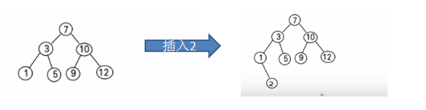
给你一个数列{1,2,3,4,5,6},要求创建一颗二叉排序树(BST), 并分析问题所在:
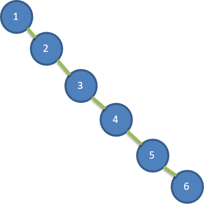
上图BST存在的问题分析:左子树全部为空,从形式上看,更像一个单链表。插入速度没有影响查询速度明显降低(因为需要依次比较), 不能发挥BST的优势,因为每次还需要比较左子树,其查询速度比单链表还慢
解决方案:平衡二叉树(AVL),对二叉排序树的优化
-
原理
平衡二叉树,也叫平衡二叉搜索树(Self-balancing binary search tree),又被称为AVL树, 可以保证查询效率较高。
具有以下特点:它是一棵空树或它的左右两个子树的高度差的绝对值不超过1,并且左右两个子树都是一棵平衡二叉树。
平衡二叉树的常用实现方法有红黑树、AVL、替罪羊树、Treap、伸展树等。
-
处理方法
注:失衡根节点,指的是左右子树高度差大于1的节点
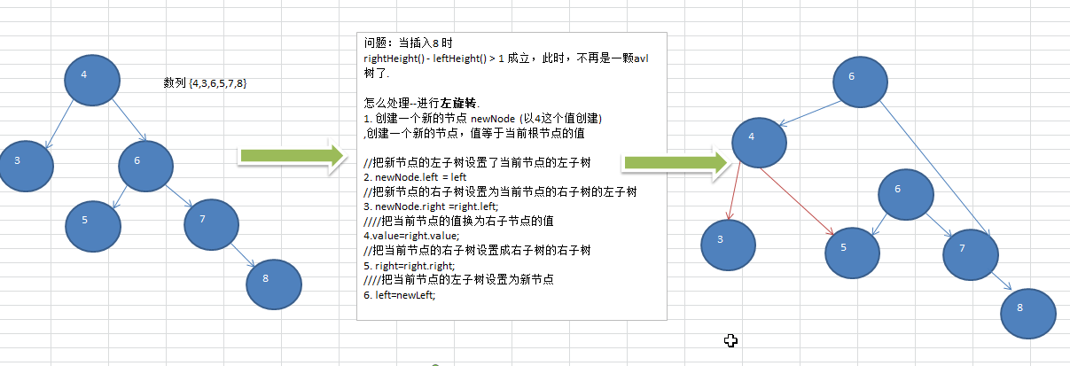
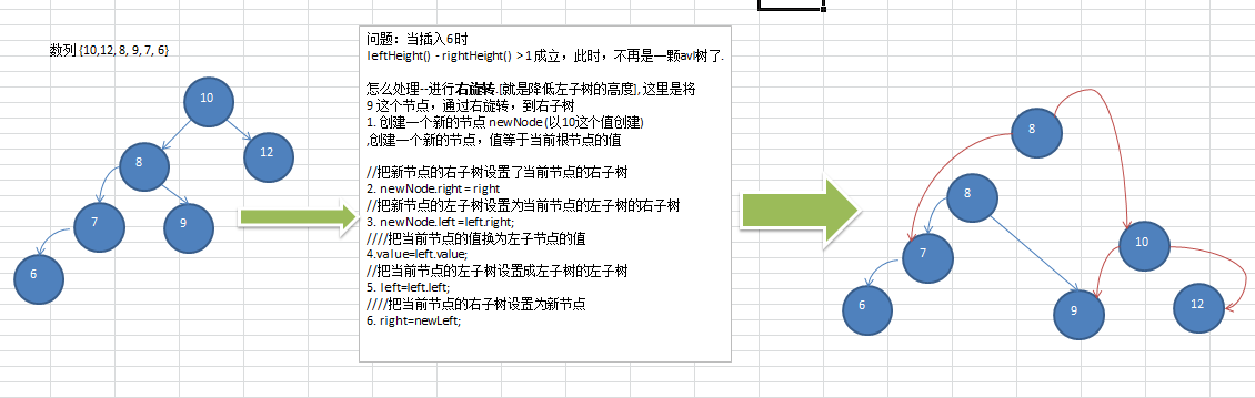
情形一:节点添加在失衡根节点的右子节点的右子节点(RR)–左旋转
情形二:节点添加在失衡根节点的左子节点的左子节点(LL)–右旋转
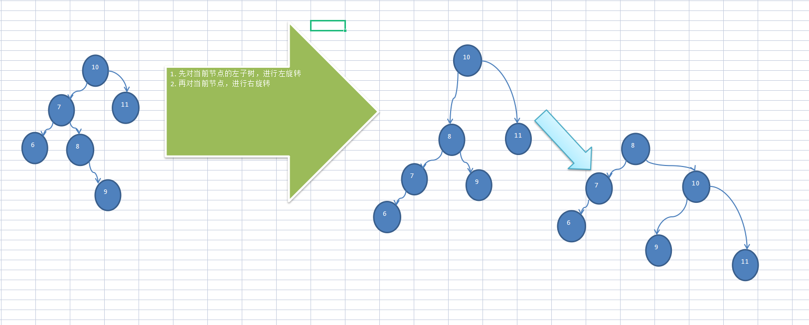
情形三:节点添加在失衡根节点的左子节点的右子节点(LR)–先以左子节点为根节点进行左旋转(局部调整平衡),再以当前节点进行右旋转
情形四:节点添加在失衡根节点的右子节点的左子节点(RL)–先以右子节点为根节点进行右旋转(局部调整平衡),再以当前节点进行左旋转
类似上图的效果
-
代码
1 2 3 4 5 6 7 8 9 10 11 12 13 14 15 16 17 18 19 20 21 22 23 24 25 26 27 28 29 30 31 32 33 34 35 36 37 38 39 40 41 42 43 44 45 46 47 48 49 50 51 52 53 54 55 56 57 58 59 60 61 62 63 64 65 66 67 68 69 70 71//class node3: //左旋转 public void leftRotate() { //创建当前根节点的副本 node3 node = new node3(this.val); //将副本左子节点指向当前节点的左子节点 node.left = this.left; //副本右子节点指向当前节点的右子节点的左子节点 node.right = this.right.left; //将当前节点的值换成右子节点的值 this.val = this.right.val; //将新的当前节点的左子节点指向副本节点 this.left = node; //将新的当前节点的右子树的右子树连接 this.right = this.right.right; } //右旋转 public void rightRotate() { node3 node = new node3(this.val); node.left = this.left.right; node.right = this.right; this.val = left.val; this.right = node; this.left = this.left.left; } //当前节点左子树高度 public int leftHeight() { if (this.left == null) return 0; return this.left.height(); } //当前节点右子树高度 public int rightHeight() { if (this.right == null) return 0; return this.right.height(); } //返回当前节点为跟节点的树的高度 public int height() {//递归查找,每递归一次树的深度+1 return Math.max((this.left == null ? 0 : this.left.height()), this.right == null ? 0 : this.right.height()) + 1; } //添加二叉排序树的节点 public void add(node3 node) { if (node == null) return; if (this.val > node.val) {//添加节点比当前节点小,向左子树处理 if (this.left == null) this.left = node; //向左子树递归 else this.left.add(node); } else {//添加节点比当前节点大,向右子树处理 if (this.right == null) this.right = node; //向右子树递归 else this.right.add(node); } //节点添加完毕,需要判断平衡因子 if (this.rightHeight() - this.leftHeight() > 1) {//右子树比左子树高,触发左旋转 //如果右子节点的左子树高度大于右子节点的右子树高度,先局部右旋转:当前节点的右子节点 if (this.right != null && this.right.leftHeight() > this.right.rightHeight()) { this.right.rightRotate(); } this.leftRotate(); } else if (this.leftHeight() - this.rightHeight() > 1) {//左子树比右子树高,触发右旋转 //如果左子节点的右子树高度大于左子节点的左子树高度,先局部左旋转:当前节点的左子节点 if (this.left != null && this.left.rightHeight() > this.left.leftHeight()) { this.left.leftRotate(); } this.rightRotate(); } }
3. B树
B-tree树即B树,B即Balanced,平衡的意思。有人把B-tree翻译成B-树,容易让人产生误解。会以为B-树是一种树,而B树又是另一种树。实际上,B-tree就是指的B树。
① 二叉树的问题分析
二叉树的操作效率较高,但是也存在问题, 请看下面的二叉树
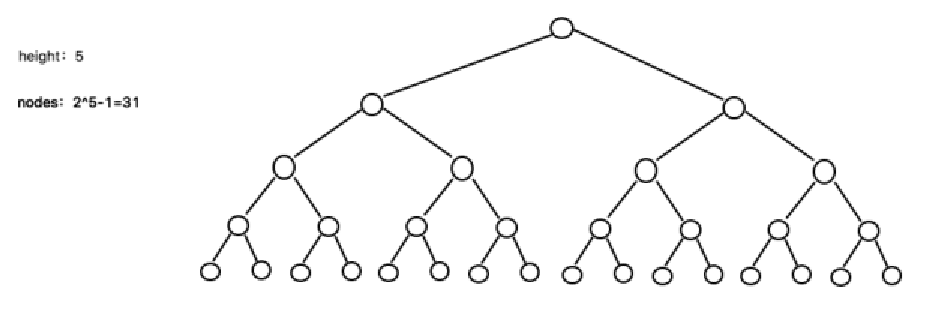
二叉树需要加载到内存的,如果二叉树的节点少,没有什么问题,但是如果二叉树的节点很多(比如1亿),就存在如下问题:
-
问题1:在构建二叉树时,需要多次进行i/o操作(海量数据存在数据库或文件中),节点海量,构建二叉树时,速度有影响
-
问题2:节点海量,也会造成二叉树的高度很大,会降低操作速度
② 多叉树
在二叉树中,每个节点有数据项,最多有两个子节点。如果允许每个节点可以有更多的数据项和更多的子节点,就是多叉树(multiway tree)
后面我们讲解的2-3树,2-3-4树就是多叉树,多叉树通过重新组织节点,减少树的高度,能对二叉树进行优化。
举例说明(下面2-3树就是一颗多叉树)
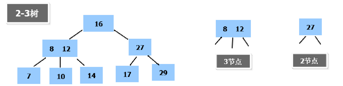
③ B树
B树通过重新组织节点,降低树的高度,并且减少i/o读写次数来提升效率。
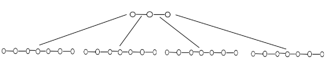
如图B树通过重新组织节点,降低了树的高度。
文件系统及数据库系统的设计者利用了磁盘预读原理,将一个节点的大小设为等于一个页(页得大小通常为4k),这样每个节点只需要一次I/O就可以完全载入
将树的度M设置为1024,在600亿个元素中最多只需要4次I/O操作就可以读取到想要的元素, B树(B+)广泛应用于文件存储系统以及数据库系统中
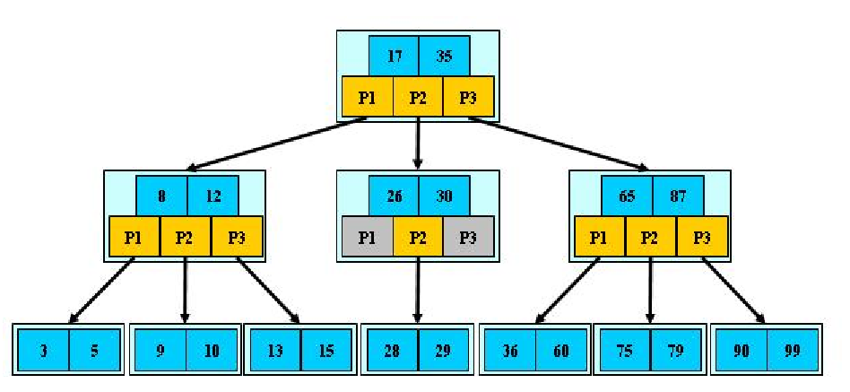
B树的说明:
-
B树的阶:节点的最多子节点个数。比如2-3树的阶是3,2-3-4树的阶是4
-
B树的搜索:从根结点开始,对结点内的关键字(有序)序列进行二分查找,如果命中则结束,否则进入查询关键字所属范围的儿子结点;重复,直到所对应的儿子指针为空,或已经是叶子结点
-
关键字集合分布在整颗树中, 即叶子节点和非叶子节点都存放数据
-
搜索有可能在非叶子结点结束
-
其搜索性能等价于在关键字全集内做一次二分查找
-
2-3树基本介绍
2-3树是最简单的B树结构, 具有如下特点:
- 2-3树的所有叶子节点都在同一层(只要是B树都满足这个条件)
- 有两个子节点的节点叫二节点,二节点要么没有子节点,要么有两个子节点
- 有三个子节点的节点叫三节点,三节点要么没有子节点,要么有三个子节点
- 2-3树是由二节点和三节点构成的树。
-
2-3树应用案例
将数列
{16, 24, 12, 32, 14, 26, 34, 10, 8, 28, 38, 20}构建成2-3树,并保证数据插入的大小顺序。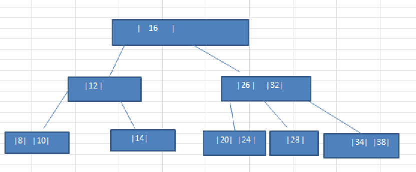
2-3树插入规则:
- 2-3树的所有叶子节点都在同一层(只要是B树都满足这个条件)
- 有两个子节点的节点叫二节点,二节点要么没有子节点,要么有两个子节点
- 有三个子节点的节点叫三节点,三节点要么没有子节点,要么有三个子节点
- 当按照规则插入一个数到某个节点时,不能满足上面三个要求,就需要拆,先向上拆,如果上层满,则拆本层,拆后仍然需要满足上面3个条件。
- 对于三节点的子树的值大小仍然遵守(BST二叉排序树)的规则
除了23树,还有234树等,概念和23树类似,也是一种B树。
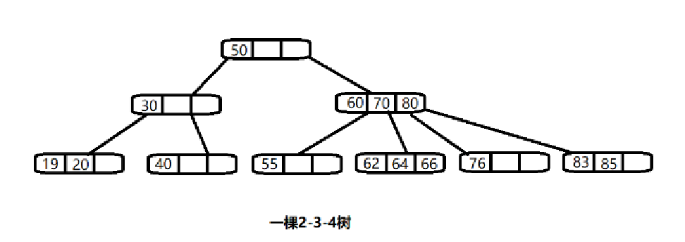
⑤ B+树
前面已经介绍了2-3树和2-3-4树,他们就是B树(英语:B-tree 也写成B-树),这里我们再做一个说明,我们在学习Mysql时,经常听到说某种类型的索引是基于B树或者B+树的,如图:
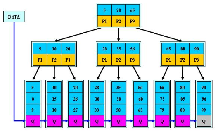
B+树的说明:
- B+树的搜索与B树也基本相同,区别是B+树只有达到叶子结点才命中(B树可以在非叶子结点命中),其性能也等价于在关键字全集做一次二分查找
- 所有关键字都出现在叶子结点的链表中(即数据只能在叶子节点【也叫稠密索引】),且链表中的关键字(数据)恰好是有序的。
- 不可能在非叶子结点命中
- 非叶子结点相当于是叶子结点的索引(稀疏索引),叶子结点相当于是存储(关键字)数据的数据层
- 更适合文件索引系统
- B树和B+树各有自己的应用场景,不能说B+树完全比B树好,反之亦然.
⑥ B*树
B*树是B+树的变体,在B+树的非根和非叶子结点再增加指向兄弟的指针。
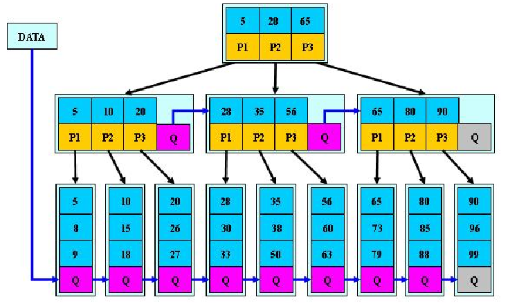
B树的说明:
-
B树定义了非叶子结点关键字个数至少为
(2/3)*M,即块的最低使用率为2/3,而B+树的块的最低使用率为B+树的1/2。 -
从第1个特点我们可以看出,B*树分配新结点的概率比B+树要低,空间使用率更高
八、图
1. 图的基本介绍
-
为什么要有图
-
线性表局限于一个直接前驱和一个直接后继的关系
-
树也只能有一个直接前驱也就是父节点
-
当我们需要表示多对多的关系时, 这里我们就用到了图
-
-
图的举例说明
图是一种数据结构,其中结点可以具有零个或多个相邻元素。两个结点之间的连接称为边。 结点也可以称为顶点。如图:
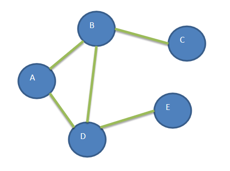
-
图的常用概念
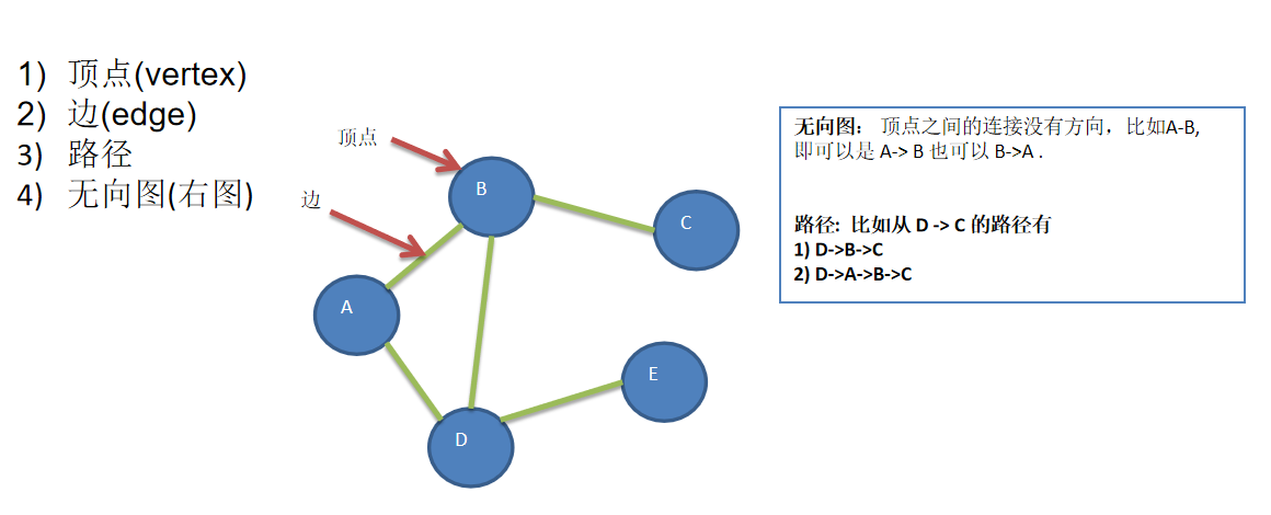
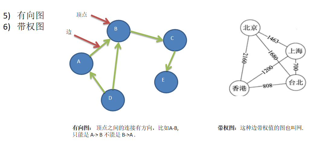
-
图的表示方式
图的表示方式有两种:二维数组表示(邻接矩阵);链表表示(邻接表)。
-
邻接矩阵
邻接矩阵是表示图形中顶点之间相邻关系的矩阵,对于n个顶点的图而言,矩阵是的row和col表示的是1~n个点。1表示直接连接,0表示不能直接连接。
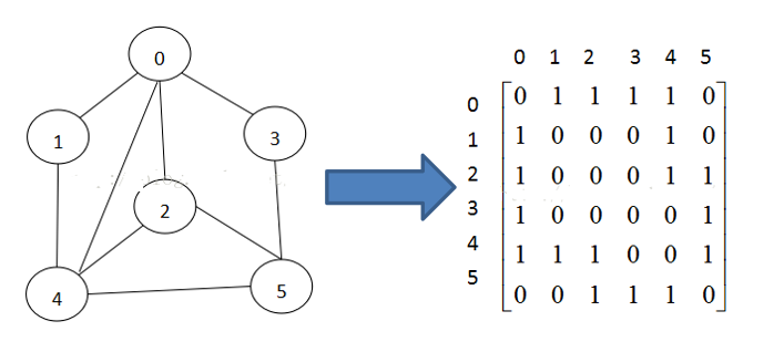
-
邻接表
邻接矩阵需要为每个顶点都分配n个边的空间,其实有很多边都是不存在,会造成空间的一定损失。邻接表的实现只关心存在的边,不关心不存在的边。因此没有空间浪费,邻接表由数组+链表组成。
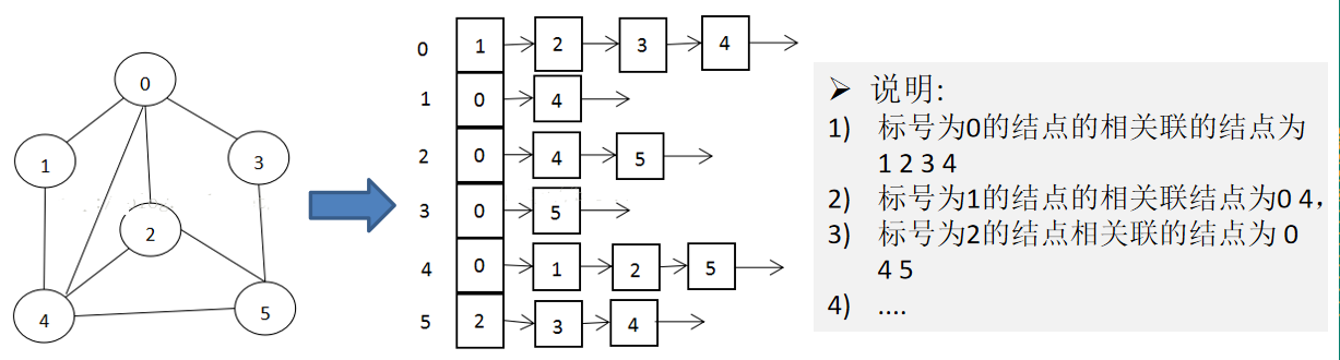
-
-
创建图
1 2 3 4 5 6 7 8 9 10 11 12 13 14 15 16 17 18 19 20 21 22 23 24 25 26 27 28 29 30 31 32 33 34 35 36 37 38 39 40 41 42 43 44 45 46 47 48 49 50 51 52 53 54 55 56 57 58 59 60 61 62 63 64 65 66 67 68 69 70 71 72 73 74 75package graph; import java.util.ArrayList; import java.util.Arrays; /* * 图 * */ public class graph { private ArrayList<String> vertexList;//存储顶点集合 private int[][] edges;//表示图对应的邻接矩阵 private int numOfEdge;//表示边的数目 public static void main(String[] args) { int n = 5; String[] vertexes = {"A", "B", "C", "D", "E"}; graph g = new graph(n); //添加顶点 for (String v : vertexes) { g.insertVertex(v); } //添加边 g.insertEdge(0, 1, 1); g.insertEdge(0, 2, 1); g.insertEdge(1, 2, 1); g.insertEdge(1, 3, 1); g.insertEdge(1, 4, 1); g.show(); } public graph(int n) { this.edges = new int[n][n]; this.numOfEdge = 0; this.vertexList = new ArrayList<>(n); } //返回节点的个数 public int getNumOfVertex() { return this.vertexList.size(); } //返回边的个数 public int getNumOfEdge() { return this.numOfEdge; } //返回节点对应的数据 public String getValueByIndex(int index) { return this.vertexList.get(index); } //返回权值 public int getWeight(int index1, int index2) { return this.edges[index1][index2]; } //插入节点 public void insertVertex(String vertex) { this.vertexList.add(vertex); } //添加边 public void insertEdge(int index1, int index2, int weight) { this.edges[index1][index2] = weight; this.edges[index2][index1] = weight; } //显示图对应的矩阵 public void show() { for (int[] v1 : this.edges) { System.out.println(Arrays.toString(v1)); } } }
2. 图的深度优先算法(DFS)
深度优先搜索类似于树的先序遍历。如其名称中所暗含的意思一样,这种搜索算法所遵循的搜索策略是尽可能“深”地搜索一个图。它的基本思想如下:首先访问图中某一起始顶点v,然后由v出发,访问与v邻接且未被访问的任一顶点w,再访问与w邻接且未被访问的任一顶点…重复上述过程。当不能再继续向下访问时,依次退回(回溯)到最近被访问的顶点,若它还有邻接顶点未被访问过,则从该点开始继续上述搜索过程,直至图中所有顶点均被访问过为止。
-
算法过程
- 访问初始结点
v,并标记结点v为已访问 - 查找结点
v的第一个邻接结点w - 若
w存在,则继续执行第4步;如果w不存在,则回到第1步,将从v的下一个结点继续 - 若
w未被访问,对w进行深度优先遍历递归(即把w当做另一个v,然后进行步骤123);若w已被访问,查找结点v的w邻接结点的下一个未访问的邻接结点,转到第3步
- 访问初始结点
-
代码实现
1 2 3 4 5 6 7 8 9 10 11 12 13 14 15 16 17 18 19 20 21 22 23 24 25 26bool visited[MAX_VERTEX_NUM]; //访问标记数组 /*从顶点出发,深度优先遍历图G*/ void DFS(Graph G, int v){ int w; visit(v); //访问顶点 visited[v] = TRUE; //设已访问标记 //FirstNeighbor(G,v):求图G中顶点v的第一个邻接点,若有则返回顶点号,否则返回-1。 //NextNeighbor(G,v,w):假设图G中顶点w是顶点v的一个邻接点,返回除w外顶点v for(w = FirstNeighbor(G, v); w>=0; w=NextNeighor(G, v, w)){ if(!visited[w]){ //w为u的尚未访问的邻接顶点 DFS(G, w); } } } /*对图进行深度优先遍历*/ void DFSTraverse(MGraph G){ int v; for(v=0; v<G.vexnum; ++v){ visited[v] = FALSE; //初始化已访问标记数据 } for(v=0; v<G.vexnum; ++v){ //从v=0开始遍历 if(!visited[v]){ DFS(G, v); } } }
3. 图的广度优先算法(BFS)
如果说图的深度优先遍历类似树的前序遍历,那么图的广度优先遍历就类似于树的层序遍历了。 广度优先搜索是一种分层的查找过程,每向前走一步可能访问一批顶点,不像深度优先搜索那样有往回退(回溯)的情况,因此它不是一个递归的算法。为了实现逐层的访问,算法必须借助一个辅助队列,以记忆正在访问的顶点(只有知道了上层顶点,才可以访问邻接的下层顶点,所以需要记录正在访问的顶点。使用一个队列以保持访问过的结点的顺序,以便按这个顺序来访问这些结点的邻接结点)。
-
算法过程
- 访问初始结点
v并标记结点v为已访问 - 结点
v入队列 - 当队列非空时,继续执行,否则算法结束
- 出队列,取得队头结点
u - 查找结点
u的第一个邻接结点w - 若结点
u的邻接结点w不存在,则转到步骤3;否则循环执行以下三个步骤:- 若结点
w尚未被访问,则访问结点w并标记为已访问 - 结点
w入队列 - 查找结点
u的继w邻接结点后的下一个邻接结点w,转到步骤6
- 若结点
- 访问初始结点
-
代码实现
1 2 3 4 5 6 7 8 9 10 11 12 13 14 15 16 17 18 19 20 21 22 23 24 25 26 27 28 29 30 31/*邻接矩阵的广度遍历算法*/ void BFSTraverse(MGraph G){ int i, j; Queue Q; for(i = 0; i<G,numVertexes; i++){ visited[i] = FALSE; } InitQueue(&Q); //初始化一辅助用的队列 for(i=0; i<G.numVertexes; i++){ //若是未访问过就处理 if(!visited[i]){ vivited[i] = TRUE; //设置当前访问过 visit(i); //访问顶点 EnQueue(&Q, i); //将此顶点入队列 //若当前队列不为空 while(!QueueEmpty(Q)){ DeQueue(&Q, &i); //顶点i出队列 //FirstNeighbor(G,v):求图G中顶点v的第一个邻接点,若有则返回顶点号,否则返回-1。 //NextNeighbor(G,v,w):假设图G中顶点w是顶点v的一个邻接点,返回除w外顶点v for(j=FirstNeighbor(G, i); j>=0; j=NextNeighbor(G, i, j)){ //检验i的所有邻接点 if(!visited[j]){ visit(j); //访问顶点j visited[j] = TRUE; //访问标记 EnQueue(Q, j); //顶点j入队列 } } } } } }
九、十大算法
1. 查找算法
2. 分治算法
① 基本概念
在计算机科学中,分治法是一种很重要的算法。字面上的解释是“分而治之”,就是把一个复杂的问题分成两个或更多的相同或相似的子问题,再把子问题分成更小的子问题……直到最后子问题可以简单的直接求解,原问题的解即子问题的解的合并。这个技巧是很多高效算法的基础,如排序算法(快速排序,归并排序),傅立叶变换(快速傅立叶变换)……
任何一个可以用计算机求解的问题所需的计算时间都与其规模有关。问题的规模越小,越容易直接求解,解题所需的计算时间也越少。例如,对于n个元素的排序问题,当n=1时,不需任何计算。n=2时,只要作一次比较即可排好序。n=3时只要作3次比较即可。而当n较大时,问题就不那么容易处理了。要想直接解决一个规模较大的问题,有时是相当困难的
② 基本思想及策略
分治法的设计思想是:将一个难以直接解决的大问题,分割成一些规模较小的相同问题,以便各个击破,分而治之。
分治策略是:对于一个规模为n的问题,若该问题可以容易地解决(比如说规模n较小)则直接解决,否则将其分解为k个规模较小的子问题,这些子问题互相独立且与原问题形式相同,递归地解这些子问题,然后将各子问题的解合并得到原问题的解。这种算法设计策略叫做分治法。
如果原问题可分割成k个子问题,1<k≤n,且这些子问题都可解并可利用这些子问题的解求出原问题的解,那么这种分治法就是可行的。由分治法产生的子问题往往是原问题的较小模式,这就为使用递归技术提供了方便。在这种情况下,反复应用分治手段,可以使子问题与原问题类型一致而其规模却不断缩小,最终使子问题缩小到很容易直接求出其解。这自然导致递归过程的产生。分治与递归像一对孪生兄弟,经常同时应用在算法设计之中,并由此产生许多高效算法。
③ 适用的情况
分治法所能解决的问题一般具有以下几个特征:
- 该问题的规模缩小到一定的程度就可以容易地解决
- 该问题可以分解为若干个规模较小的相同问题,即该问题具有最优子结构性质
- 利用该问题分解出的子问题的解可以合并为该问题的解
- 该问题所分解出的各个子问题是相互独立的,即子问题之间不包含公共的子子问题
第一条特征是绝大多数问题都可以满足的,因为问题的计算复杂性一般是随着问题规模的增加而增加
第二条特征是应用分治法的前提,它也是大多数问题可以满足的,此特征反映了递归思想的应用
第三条特征是关键,能否利用分治法完全取决于问题是否具有第三条特征,如果具备了第一条和第二条特征,而不具备第三条特征,则可以考虑用贪心法或动态规划法
第四条特征涉及到分治法的效率,如果各子问题是不独立的则分治法要做许多不必要的工作,重复分解公共的子问题,此时虽然可用分治法,但一般用动态规划法较好
④ 基本步骤
分治法在每一层递归上都有三个步骤:
- 分解:将原问题分解为若干个规模较小,相互独立,与原问题形式相同的子问题;
- 解决:若子问题规模较小而容易被解决则直接解决,否则递归地解决各个子问题
- 合并:将各个子问题的解合并为原问题的解。
它的一般的算法设计模式如下:
Divide-and-Conquer(P):
- if |P|<=n~0~
- then return(ADHOC(P))
- 将P分解为较小的子问题 P~1~ ,P~2~ ,…,P~k~
- for i ← 1 to k
- do y~i~ ← Divide-and-Conquer(P~i~) 递归解决P~i~
- T ← MERGE(y~1~,y~2~,…,y~k~) 合并子问题
- return(T)
其中|P|表示问题P的规模;n~0~为一阈值,表示当问题P的规模不超过n~0~时,问题已容易直接解出,不必再继续分解。ADHOC(P)是该分治法中的基本子算法,用于直接解小规模的问题P。因此,当P的规模不超过n0时直接用算法ADHOC(P)求解。算法MERGE(y~1~,y~2~,…,y~k~)是该分治法中的合并子算法,用于将P的子问题P~1~ ,P~2~ ,…,P~k~的相应的解y~1~,y~2~,…,y~k~合并为P的解。
⑤ 复杂性分析
一个分治法将规模为n的问题分成k个规模为n/m的子问题去解。设分解阀值n0=1,且ADHOC(基本子算法)解规模为1的问题耗费1个单位时间。再设将原问题分解为k个子问题以及用merge将k个子问题的解合并为原问题的解需用f(n)个单位时间。用T(n)表示该分治法解规模为|P| = n的问题所需的计算时间,则有:
T(n)= k T(n/m)+f(n)
通过迭代法求得方程的解:
递归方程及其解只给出n等于m的方幂时T(n)的值,但是如果认为T(n)足够平滑,那么由n等于m的方幂时T(n)的值可以估计T(n)的增长速度。通常假定T(n)是单调上升的,从而当mi≤n<mi+1时,T(mi)≤T(n)<T(mi+1)。
⑥ 分治法求解的一些经典问题
- 二分搜索
- 大整数乘法
- Strassen矩阵乘法
- 棋盘覆盖
- 合并排序
- 快速排序
- 线性时间选择
- 最接近点对问题
- 循环赛日程表
- 汉诺塔
⑦ 依据分治法设计程序时的思维过程
实际上就是类似于数学归纳法,找到解决本问题的求解方程公式,然后根据方程公式设计递归程序。
- 一定是先找到最小问题规模时的求解方法
- 然后考虑随着问题规模增大时的求解方法
- 找到求解的递归函数式后(各种规模或因子),设计递归程序即可。
⑧ 案例
汉诺塔
-
题目
汉诺塔:汉诺塔(又称河内塔)问题是源于印度一个古老传说的益智玩具。大梵天创造世界的时候做了三根金刚石柱子,在一根柱子上从下往上按照大小顺序摞着64片黄金圆盘。大梵天命令婆罗门把圆盘从下面开始按大小顺序重新摆放在另一根柱子上。并且规定,在小圆盘上不能放大圆盘,在三根柱子之间一次只能移动一个圆盘。
-
代码
1 2 3 4 5 6 7 8 9 10 11 12 13 14 15 16 17 18 19 20 21 22package algorithm.dac; public class hanoitower { public static void main(String[] args) { move(5, 'A', 'B', 'C'); } //将第num个盘从a移到c处,中间借助b public static void move(int num, char a, char b, char c) { if (num == 1) { System.out.println("第" + num + "个盘从 " + a + "->" + c); return; } //先将最上面的所有盘,从a移动b move(num - 1, a, c, b); //把最下边的盘,从a移动到c System.out.println("第" + num + "个盘从 " + a + "->" + c); // move(1,a,b,c); //再把b塔所有盘,从b移动至c,借助a塔 move(num - 1, b, a, c); } }
3. 动态规划
① 算法的核心
理解一个算法就要理解一个算法的核心,动态规划算法的核心是一个小故事。
|
|
由上面的小故事可以知道动态规划算法的核心就是记住已经解决过的子问题的解。
② 算法的两种形式
上面已经知道动态规划算法的核心是记住已经求过的解,记住求解的方式有两种:①自顶向下的备忘录法 ②自底向上。 为了说明动态规划的这两种方法,举一个最简单的例子:求斐波拉契数列**Fibonacci **。先看一下这个问题:
|
|
以前学c语言的时候写过这个算法使用递归十分的简单。先使用递归版本来实现这个算法:
|
|
先来分析一下递归算法的执行流程,假如输入6,那么执行的递归树如下:
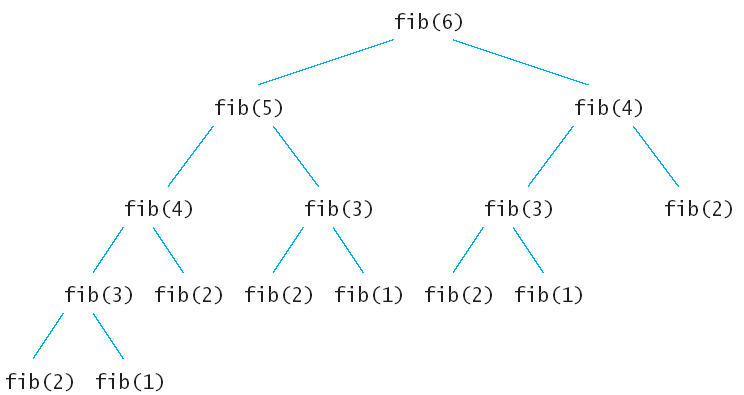 上面的递归树中的每一个子节点都会执行一次,很多重复的节点被执行,
fib(2)被重复执行了5次。由于调用每一个函数的时候都要保留上下文,所以空间上开销也不小。这么多的子节点被重复执行,如果在执行的时候把执行过的子节点保存起来,后面要用到的时候直接查表调用的话可以节约大量的时间。下面就看看动态规划的两种方法怎样来解决斐波拉契数列**Fibonacci **数列问题。
自顶向下的备忘录法
|
|
备忘录法也是比较好理解的,创建了一个n+1大小的数组来保存求出的斐波拉契数列中的每一个值,在递归的时候如果发现前面fib(n)的值计算出来了就不再计算,如果未计算出来,则计算出来后保存在Memo数组中,下次在调用fib(n)的时候就不会重新递归了。比如上面的递归树中在计算fib(6)的时候先计算fib(5),调用fib(5)算出了fib(4)后,fib(6)再调用fib(4)就不会在递归fib(4)的子树了,因为fib(4)的值已经保存在Memo[4]中。
暴力递归之中有很多节点需要重复计算,为了减少重复计算,需要使用一个缓存表(一般是一位或二位数组)记录当前递归节点的结果,以后需要再次使用时,无需递归,直接从缓存里拿结果,从而提升速度。即记忆化搜索
自底向上的动态规划
备忘录法还是利用了递归,上面算法不管怎样,计算fib(6)的时候最后还是要计算出fib(1),fib(2),fib(3)……,那么何不先计算出fib(1),fib(2),fib(3)……呢?这也就是动态规划的核心,先计算子问题,再由子问题计算父问题。
动态规划算法与分治算法类似,其基本思想也是将待求解问题分解成若干个子问题,先求解子问题,然后从这些子问题的解得到原问题的解。
与分治法不同的是,适合于用动态规划求解的问题,经分解得到子问题往往不是互相独立的。 ( 即下一个子阶段的求解是建立在上一个子阶段的解的基础上,进行进一步的求解 )
动态规划可以通过填表的方式来逐步推进,得到最优解
|
|
自底向上方法也是利用数组保存了先计算的值,为后面的调用服务。观察参与循环的只有 i,i-1 , i-2三项,因此该方法的空间可以进一步的压缩如下。
|
|
一般来说由于备忘录方式的动态规划方法使用了递归,递归的时候会产生额外的开销,使用自底向上的动态规划方法要比备忘录方法好。
③ 案例
01背包问题
-
题目
背包问题:有一个背包,容量为4磅,现有如下物品。要求达到的目标为装入的背包的总价值最大,并且重量不超出要求装入的物品不能重复
物品 重量 价格 吉他(G) 1 1500 音响(S) 4 3000 电脑(L) 3 2000 -
思路
背包问题主要是指一个给定容量的背包、若干具有一定价值和重量的物品,如何选择物品放入背包使物品的价值最大。其中又分01背包和完全背包(完全背包指的是:每种物品都有无限件可用)这里的问题属于01背包,即每个物品最多放一个。而无限背包可以转化为01背包。
算法的主要思想,利用动态规划来解决。每次遍历到的第
i个物品,根据w[i]和v[i]来确定是否需要将该物品放入背包中。即对于给定的n个物品,设v[i]、w[i]分别为第i个物品的价值和重量,C为背包的容量。再令v[i][j]表示在前i个物品中能够装入容量为j的背包中的最大价值。则我们有下面的结果:物品 0 磅 1磅 2磅 3磅 4磅 0 0 0 0 0 吉他(G) 0 1500(G) 1500(G) 1500(G) 1500(G) 音响(S) 0 1500(G) 1500(G) 1500(G) 3000(S) 电脑(L) 0 1500(G) 1500(G) 2000(L) 3500(L+G) 1 2 3 4 5 6 7 8 9(1) v[i][0]=v[0][j]=0; //表示 填入表 第一行和第一列是0 (2) 当w[i]> j 时:v[i][j]=v[i-1][j] //当准备加入新增的商品的容量大于当前背包的容量时,就直接使用上一个单元格的装入策略 (3) 当j>=w[i]时: v[i][j]=max{v[i-1][j], v[i]+v[i-1][j-w[i]]} //当准备加入的新增的商品的容量小于等于当前背包的容量, // 装入的方式: v[i-1][j] : 就是上一个单元格的装入的最大值 v[i] : 表示当前商品的价值 v[i-1][j-w[i]] : 装入i-1商品,到剩余空间j-w[i]的最大值 当j>=w[i]时 : v[i][j]=max{v[i-1][j], v[i]+v[i-1][j-w[i]]} -
代码
1 2 3 4 5 6 7 8 9 10 11 12 13 14 15 16 17 18 19 20 21 22 23 24 25 26 27 28 29 30 31 32 33 34 35 36 37 38 39 40 41 42 43 44 45 46 47 48 49 50 51 52 53package algorithm.DP; import java.util.Arrays; /* * 01背包问题 * */ public class backpackProblem { public static void main(String[] args) { //创建表 int[][] v = new int[4][5];//前i个物品中能够装入容量为j的背包中的最大价值 int[] w = new int[4];//第i个物品重量 w[1] = 1; w[2] = 4; w[3] = 3; int[] a = new int[4];//物品第i个物品单价 a[1] = 1500; a[2] = 3000; a[3] = 2000; //开始决策填表 //填充第一列 int rowNum = v.length; for (int i = 0; i < rowNum; i++) { v[i][0] = 0; } //填充第一行 int colNum = v[0].length; for (int j = 0; j < colNum; j++) { v[0][j] = 0; } //填充第二行:只能放第一个商品 for (int j = 0; j < colNum; j++) { if (w[1] <= j) v[1][j] = a[1]; } //决策其他单元格 for (int i = 2; i < rowNum; i++) { for (int j = 1; j < colNum; j++) { //当前物品放不下,只有依赖上次决策的结果 if (w[i] > j) v[i][j] = v[i - 1][j]; //当前物品放得下,需要比较将当前物品放入之后再填放以前物品的加之和不放当前物品的价值 else v[i][j] = Math.max(v[i - 1][j], a[i] + v[i - 1][j - w[i]]); } } for (int i = 0; i < rowNum; i++) { System.out.println(Arrays.toString(v[i])); System.out.println(); } } }
4. KMP算法
① 暴力匹配算法
假设现在我们面临这样一个问题:有一个文本串S,和一个模式串P,现在要查找P在S中的位置,怎么查找呢?
如果用暴力匹配的思路,并假设现在文本串S匹配到 i 位置,模式串P匹配到 j 位置,则有:
-
如果当前字符匹配成功(即
S[i] == P[j]),则i++,j++,继续匹配下一个字符; -
如果失配(即
S[i]! = P[j]),令i = i - (j - 1),j = 0。相当于每次匹配失败时,i回溯,j被置为0。理清楚了暴力匹配算法的流程及内在的逻辑,咱们可以写出暴力匹配的代码,如下:
|
|
举个例子,如果给定文本串S:“BBC ABCDAB ABCDABCDABDE”,和模式串P:“ABCDABD”,现在要拿模式串P去跟文本串S匹配,整个过程如下所示:
-
S[0]为B,P[0]为A,不匹配,执行第②条指令:“如果失配(即S[i]! = P[j]),令i = i - (j - 1),j = 0"。S[1]跟P[0]匹配,相当于模式串要往右移动一位(i=1,j=0)
-
S[1]跟P[0]还是不匹配,继续执行第②条指令:“如果失配(即S[i]! = P[j]),令i = i - (j - 1),j = 0”,S[2]跟P[0]匹配(i=2,j=0),从而模式串不断的向右移动一位(不断的执行“令i = i - (j - 1),j = 0”,i从2变到4,j一直为0)
-
直到
S[4]跟P[0]匹配成功(i=4,j=0),此时按照上面的暴力匹配算法的思路,转而执行第①条指令:“如果当前字符匹配成功(即S[i] == P[j]),则i++,j++”,可得S[i]为S[5],P[j]为P[1],即接下来S[5]跟P[1]匹配(i=5,j=1)
-
S[5]跟P[1]匹配成功,继续执行第①条指令:“如果当前字符匹配成功(即S[i] == P[j]),则i++,j++”,得到S[6]跟P[2]匹配(i=6,j=2),如此进行下去
-
直到
S[10]为空格字符,P[6]为字符D(i=10,j=6),因为不匹配,重新执行第②条指令:“如果失配(即S[i]! = P[j]),令i = i - (j - 1),j = 0”,相当于S[5]跟P[0]匹配(i=5,j=0)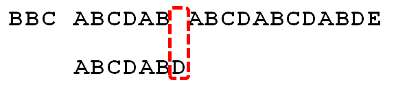
-
至此,我们可以看到,如果按照暴力匹配算法的思路,尽管之前文本串和模式串已经分别匹配到了
S[9]、P[5],但因为S[10]跟P[6]不匹配,所以文本串回溯到S[5],模式串回溯到P[0],从而让S[5]跟P[0]匹配。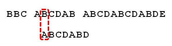
而
S[5]肯定跟P[0]失配。为什么呢?因为在之前第4步匹配中,我们已经得知S[5] = P[1] = B,而P[0] = A,即P[1] != P[0],故S[5]必定不等于P[0],所以回溯过去必然会导致失配。那有没有一种算法,让i不往回退,只需要移动j即可呢?答案是肯定的。这种算法就是本文的主旨KMP算法,它利用之前已经部分匹配这个有效信息,保持
i不回溯,通过修改j的位置,让模式串尽量地移动到有效的位置。
② KMP算法
定义
下面先直接给出KMP的算法流程
- 假设现在文本串S匹配到 i 位置,模式串P匹配到j位置
- 如果j = -1,或者当前字符匹配成功(即S[i] == P[j]),都令i++,j++,继续匹配下一个字符;
- 如果j != -1,且当前字符匹配失败(即S[i] != P[j]),则令 i 不变,j = next[j]。此举意味着失配时,模式串P相对于文本串S向右移动了j - next [j] 位。(注意:是相对,文本串没有移动,只是将模式串的j指针往前(向左)移动到next[j]位置,因此相对文本串来说:模式串S向右移动了j-next[j]位)
- 换言之,当匹配失败时,模式串向右移动的位数为:失配字符所在位置 - 失配字符对应的next值),即移动的实际位数为:j - next[j],且此值大于等于1。
很快,你也会意识到next 数组各值的含义:代表当前字符之前的字符串中,有多大长度的相同前缀后缀。例如如果next [j] = k,代表j 之前的字符串中有最大长度为k 的相同前缀后缀。
此也意味着在某个字符失配时,该字符对应的next 值会告诉你下一步匹配中,模式串应该跳到哪个位置(跳到next [j] 的位置)。如果next [j] 等于0或-1,则跳到模式串的开头字符,若next [j] = k 且 k > 0,代表下次匹配跳到j 之前的某个字符,而不是跳到开头,且具体跳过了k 个字符。
步骤
-
寻找前缀后缀最长公共元素长度
对于P= p~0~,p~1~…p~j-1~,p~j~,寻找模式串P中长度最大且相等的前缀和后缀。如果存在p~0~,p~1~ …p~k-1~,p~k~ = p~j-k~,p~j-k+1~…p~j-1~,p~j~,那么在包含p~j~的模式串中有最大长度为k+1的相同前缀后缀。举个例子,如果给定的模式串为“abab”,那么它的各个子串的前缀后缀的公共元素的最大长度如下表格所示:
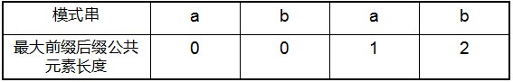 比如对于字符串aba来说,它有长度为1的相同前缀后缀a;而对于字符串abab来说,它有长度为2的相同前缀后缀ab(相同前缀后缀的长度为k + 1,k + 1 = 2)。
 -
根据前缀后缀最长公共元素长度,求next数组(也可以不求,直接根据最大长度表得出结果)
将第①步骤中求得的值整体右移一位,然后初值赋为-1,即结果
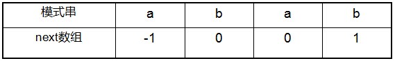
-
根据next数组进行匹配
匹配失配,j = next [j],模式串向右移动的位数为:j - next[j]。换言之,当模式串的后缀p~j-k~,p~j-k+1~, …, p~j-1~ 跟文本串 s~i-k~,s~i-k+1~, …, s~i-1~匹配成功,但 p~j~ 跟 s~i~ 匹配失败时,因为next[j] = k,相当于在不包含 p~j~ 的模式串中有最大长度为 k 的相同前缀后缀,即p~0~,p~1~ …p~k-1~ = p~j-k~,p~j-k+1~…p~j-1~,故令j = next[j],从而让模式串右移j - next[j] 位,使得模式串的前缀p~0~,p~1~…p~k-1~对应着文本串 s~i-k~,s~i-k+1~…s~i-1~,而后让p~k~跟s~i~继续匹配。如下图所示:
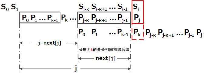
综上,KMP的next 数组相当于告诉我们:当模式串中的某个字符跟文本串中的某个字符匹配失配时,模式串下一步应该跳到哪个位置。如模式串中在j 处的字符跟文本串在i 处的字符匹配失配时,下一步用next [j] 处的字符继续跟文本串i 处的字符匹配,相当于模式串向右移动 j - next[j] 位。
代码
|
|
5. 贪心算法
① 基本概念
所谓贪心算法是指,在对问题求解时,总是做出在当前看来是最好的选择。也就是说,不从整体最优上加以考虑,它所做出的仅仅是在某种意义上的局部最优解。 贪心算法没有固定的算法框架,算法设计的关键是贪心策略的选择。必须注意的是,贪心算法不是对所有问题都能得到整体最优解,选择的贪心策略必须具备无后效性(即某个状态以后的过程不会影响以前的状态,只与当前状态有关。) 所以,对所采用的贪心策略一定要仔细分析其是否满足无后效性。
② 贪心算法的基本思路
- 建立数学模型来描述问题
- 把求解的问题分成若干个子问题
- 对每个子问题求解,得到子问题的局部最优解
- 把子问题的解局部最优解合成原来问题的一个解
③ 该算法存在的问题
- 不能保证求得的最后解是最佳的
- 不能用来求最大值或最小值的问题
- 只能求满足某些约束条件的可行解的范围
④ 贪心算法适用的问题
贪心策略适用的前提是:局部最优策略能导致产生全局最优解。 实际上,贪心算法适用的情况很少。一般对一个问题分析是否适用于贪心算法,可以先选择该问题下的几个实际数据进行分析,就可以做出判断。
⑤ 贪心选择性质
所谓贪心选择性质是指所求问题的整体最优解可以通过一系列局部最优的选择,换句话说,当考虑做何种选择的时候,我们只考虑对当前问题最佳的选择而不考虑子问题的结果。这是贪心算法可行的第一个基本要素。贪心算法以迭代的方式作出相继的贪心选择,每作一次贪心选择就将所求问题简化为规模更小的子问题。对于一个具体问题,要确定它是否具有贪心选择性质,必须证明每一步所作的贪心选择最终导致问题的整体最优解。 当一个问题的最优解包含其子问题的最优解时,称此问题具有最优子结构性质。问题的最优子结构性质是该问题可用贪心算法求解的关键特征。
⑥ 贪心算法的实现框架
从问题的某一初始解出发: while (朝给定总目标前进一步) { 利用可行的决策,求出可行解的一个解元素。 } 由所有解元素组合成问题的一个可行解;
⑦ 例题分析
【背包问题】有一个背包,容量是M=150,有7个物品,物品可以分割成任意大小。要求尽可能让装入背包中的物品总价值最大,但不能超过总容量。
物品: 重量:35 30 60 50 40 10 25 价值:10 40 30 50 35 40 30
分析: 目标函数: ∑p~i~最大 约束条件是装入的物品总质量不超过背包容量:∑w~i~<=M( M=150) (1)根据贪心的策略,每次挑选价值最大的物品装入背包,得到的结果是否最优? (2)每次挑选所占重量最小的物品装入是否能得到最优解? (3)每次选取单位重量价值最大的物品,成为解本题的策略
值得注意的是,贪心算法并不是完全不可以使用,贪心策略一旦经过证明成立后,它就是一种高效的算法。比如,求最小生成树的Prim算法和Kruskal算法都是漂亮的贪心算法。 贪心算法还是很常见的算法之一,这是由于它简单易行,构造贪心策略不是很困难。 可惜的是,它需要证明后才能真正运用到题目的算法中。 一般来说,贪心算法的证明围绕着:整个问题的最优解一定由在贪心策略中存在的子问题的最优解得来的。 对于例题中的3种贪心策略,都是无法成立(无法被证明)的,解释如下: 贪心策略:选取价值最大者。
反例:
W=30
物品:A B C
重量:28 12 12
价值:30 20 20
根据策略,首先选取物品A,接下来就无法再选取了,可是,选取B、C则更好。
(2)贪心策略:选取重量最小。它的反例与第一种策略的反例差不多。
(3)贪心策略:选取单位重量价值最大的物品。反例:
W=30
物品:A B C
重量:28 20 10
价值:28 20 10
根据策略,三种物品单位重量价值一样,程序无法依据现有策略作出判断,如果选择A,则答案错误。但是果在条件中加一句当遇见单位价值相同的时候,优先装重量小的,这样的问题就可以解决.
所以需要说明的是,贪心算法可以与随机化算法一起使用,具体的例子就不再多举了。(因为这一类算法普及性不高,而且技术含量是非常高的,需要通过一些反例确定随机的对象是什么,随机程度如何,但也是不能保证完全正确,只能是极大的几率正确)
6. 最小生成树(MST)
-
定义:
在给定一张无向图,如果在它的子图中,任意两个顶点都是互相连通,并且是一个树结构,那么这棵树叫做生成树。当连接顶点之间的图有权重时,权重之和最小的树结构为最小生成树!
-
性质:
-
给定一个带权的无向连通图,如何选取一棵生成树,使树上所有边上权的总和为最小,这叫最小生成树
-
N个顶点,一定有N-1条边
-
包含全部顶点N-1条边都在图中
-
举例说明(如图:)
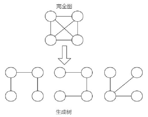
-
求最小生成树的算法主要是普里姆算法和克鲁斯卡尔算法
-
① Prim算法(普里姆算法)
Prim算法是另一种贪心算法,和Kuskral算法的贪心策略不同,Kuskral算法主要对边进行操作,而Prim算法则是对节点进行操作,每次遍历添加一个点,这时候我们就不需要使用并查集了。具体步骤为:
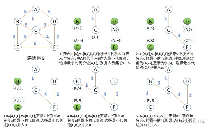
- 设G=(V,E)是连通网,T=(U,D)是最小生成树,V,U是顶点集合,E,D是边的集合
- 若从顶点u开始构造最小生成树,则从集合V中取出顶点u放入集合U中,标记顶点v的visited[u]=1
- 若集合U中顶点u~i~与集合V-U中的顶点v~j~之间存在边,则寻找这些边中权值最小的边,但不能构成回路,将顶点v~j~加入集合U中,将边(u~i~,v~j~)加入集合D中,标记visited[v~j~]=1
- 重复步骤②,直到U与V相等,即所有顶点都被标记为访问过,此时D中有n-1条边
注意:对于单连通,从一个节点出发就可以直接找到完整的最小生成树,因此最外的for循环也可以为一个顺序结构,但多连通,就需要从不同的节点出发了!!!
代码实现:
|
|
② Kruskal算法(克鲁斯卡尔算法)
在含有n个顶点的连通图中选择n-1条边,构成一棵极小连通子图,并使该连通子图中n-1条边上权值之和达到最小,则称其为连通网的最小生成树。
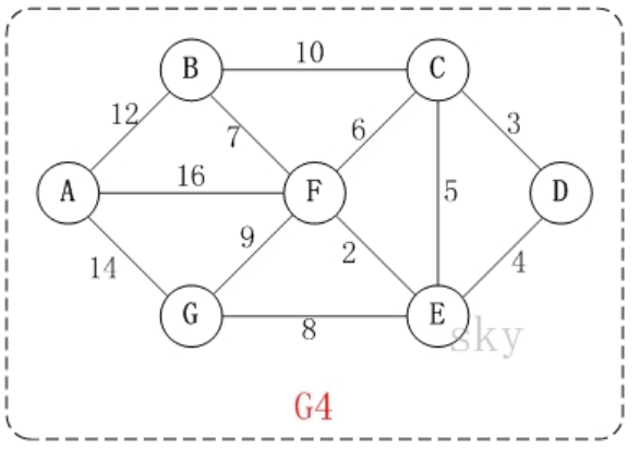
例如,对于如上图G4所示的连通网可以有多棵权值总和不相同的生成树。
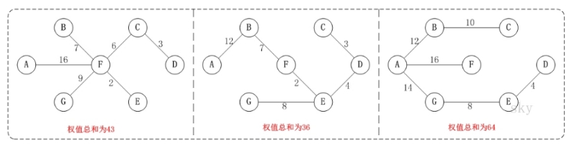
克鲁斯卡尔算法图解
以上图G4为例,来对克鲁斯卡尔进行演示(假设,用数组R保存最小生成树结果)。
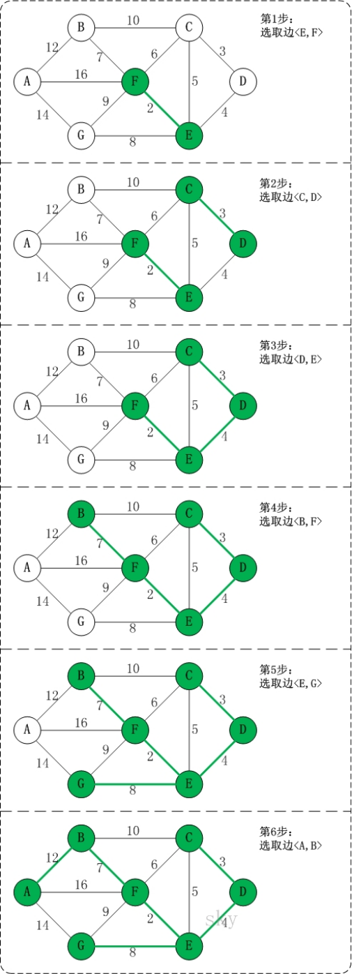
第1步:将边<E,F>加入R中。 边<E,F>的权值最小,因此将它加入到最小生成树结果R中。 第2步:将边<C,D>加入R中。 上一步操作之后,边<C,D>的权值最小,因此将它加入到最小生成树结果R中。 第3步:将边<D,E>加入R中。 上一步操作之后,边<D,E>的权值最小,因此将它加入到最小生成树结果R中。 第4步:将边<B,F>加入R中。 上一步操作之后,边<C,E>的权值最小,但<C,E>会和已有的边构成回路;因此,跳过边<C,E>。同理,跳过边<C,F>。将边<B,F>加入到最小生成树结果R中。 第5步:将边<E,G>加入R中。 上一步操作之后,边<E,G>的权值最小,因此将它加入到最小生成树结果R中。 第6步:将边<A,B>加入R中。 上一步操作之后,边<F,G>的权值最小,但<F,G>会和已有的边构成回路;因此,跳过边<F,G>。同理,跳过边<B,C>。将边<A,B>加入到最小生成树结果R中。
此时,最小生成树构造完成!它包括的边依次是:<E,F> <C,D> <D,E> <B,F> <E,G> <A,B>。
克鲁斯卡尔算法分析
根据前面介绍的克鲁斯卡尔算法的基本思想和做法,我们能够了解到,克鲁斯卡尔算法重点需要解决的以下两个问题: 问题一 对图的所有边按照权值大小进行排序。 问题二 将边添加到最小生成树中时,怎么样判断是否形成了回路。
问题一很好解决,采用排序算法进行排序即可。
问题二,实现克鲁斯卡尔算法的难点在于“如何判断一个新边是否会和已选择的边构成环路”,有一种判断的方法:
初始状态下,为连通网中的各个顶点配置不同的标记。对于一个新边,如果它两端顶点的标记不同,就不会构成环路,可以组成最小生成树。一旦新边被选择,需要将它的两个顶点以及和它直接相连的所有已选边两端的顶点改为相同的标记;反之,如果新边两端顶点的标记相同,就表示会构成环路。
代码:
|
|
7. 最短路径
① Dijkstra算法(迪杰斯特拉算法)
看一个应用场景和问题:
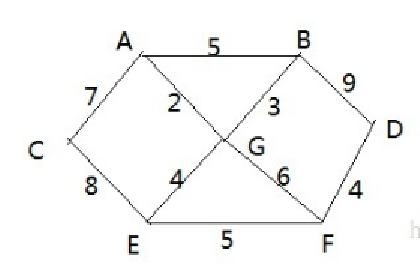
战争时期,胜利乡有7个村庄(A, B, C, D, E, F, G) ,现在有六个邮差,从G点出发,需要分别把邮件分别送到 A, B, C , D, E, F 六个村庄各个村庄的距离用边线表示(权) ,比如 A – B 距离 5公里问:如何计算出G村庄到 其它各个村庄的最短距离? 如果从其它点出发到各个点的最短距离又是多少?
**介绍: **
迪杰斯特拉(Dijkstra)算法是典型最短路径算法,用于计算一个结点到其他结点的最短路径。 它的主要特点是以起始点为中心向外层层扩展(广度优先搜索思想),直到扩展到终点为止。
算法过程:
设置出发顶点为v,顶点集合V{v1,v2,vi…},v到V中各顶点的距离构成距离集合Dis,Dis{d1,d2,di…},Dis集合记录着v到图中各顶点的距离(到自身可以看作0,v到vi距离对应为di)
- 从Dis中选择值最小的di并移出Dis集合,同时移出V集合中对应的顶点vi,此时的v到vi即为最短路径
- 更新Dis集合,更新规则为:比较v到V集合中顶点的距离值,与v通过vi到V集合中顶点的距离值,保留值较小的一个(同时也应该更新顶点的前驱节点为vi,表明是通过vi到达的)
- 重复执行两步骤,直到最短路径顶点为目标顶点即可结束
代码:
|
|
② Floyd算法(弗洛伊德算法)
- 用来求图中所有点对之间的最短路径
- Dijkstra算法是求单源最短路径的,那如果求图中所有点对的最短路径的话则有以下两种解法:
- 解法一: 以图中的每个顶点作为源点,调用Dijkstra算法,时间复杂度为O(n^3^);
- 解法二: Floyd(弗洛伊德算法)更简洁,算法复杂度仍为O(n^3^)。
- 正如大多数教材中所讲到的,求单源点无负边最短路径用Dijkstra,而求所有点最短路径用Floyd。确实,我们将用到Floyd算法,但是,并不是说所有情况下Floyd都是最佳选择。
- 对于没有学过Floyd的人来说,在掌握了Dijkstra之后遇到All-Pairs最短路径问题的第一反应可能会是:计算所有点的单源点最短路径,不就可以得到所有点的最短路径了吗。简单得描述一下算法就是执行n次Dijkstra算法。
- Floyd可以说是Warshall算法的扩展了,三个for循环便可以解决一个复杂的问题,应该说是十分经典的。从它的三层循环可以看出,它的复杂度是n^3^,除了在第二层for中加点判断可以略微提高效率,几乎没有其他办法再减少它的复杂度。
- 比较两种算法,不难得出以下的结论:对于稀疏的图,采用n次Dijkstra比较出色,对于茂密的图,可以使用Floyd算法。另外,Floyd可以处理带负边的图。
下面对Floyd算法进行介绍:
- Floyd算法的基本思想: 可以将问题分解: 第一、先找出最短的距离 第二、然后在考虑如何找出对应的行进路线。 如何找出最短路径呢,这里还是用到动态规划的知识,对于任何一个城市而言,i到j的最短距离不外乎存在经过i与j之间经过k和不经过k两种可能,所以可以令k=1,2,3,…,n(n是城市的数目),在检查d(ij)与d(ik)+d(kj)的值;在此d(ik)与d(kj)分别是目前为止所知道的i到k与k到j的最短距离,因此d(ik)+d(kj)就是i到j经过k的最短距离。所以,若有d(ij)>d(ik)+d(kj),就表示从i出发经过k再到j的距离要比原来的i到j距离短,自然把i到j的d(ij)重写为d(ik)+d(kj),每当一个k查完了,d(ij)就是目前的i到j的最短距离。重复这一过程,最后当查完所有的k时,d(ij)里面存放的就是i到j之间的最短距离了。
Floyd算法的基本步骤:
-
定义n×n的方阵序列D~-1~, D~0~ , … D~n-1~,
-
初始化: D~-1~=C
- D~-1~[i][j]=边<i,j>的长度,表示初始的从i到j的最短路径长度,即它是从i到j的中间不经过其他中间点的最短路径。
-
迭代:设D~k-1~已求出,如何得到D~k~(0≤k≤n-1)?
- D~k-1~[i][j]表示从i到j的中间点不大于k-1的最短路径p:i…j,
- 考虑将顶点k加入路径p得到顶点序列q:i…k…j,
- 若q不是路径,则当前的最短路径仍是上一步结果:D~k~[i][j]= D~k-1~[i][j];
- 否则若q的长度小于p的长度,则用q取代p作为从i到j的最短路径
-
因为q的两条子路径i…k和k…j皆是中间点不大于k-1的最短路径,所以从i到j中间点不大于k的最短路径长度为:
D~k~[i][j]=min{ D~k-1~[i][j], D~k-1~[i][k] + D~k-1~[k][j] }
Floyd算法实现:
-
可以用三个for循环把问题搞定了,但是有一个问题需要注意,那就是for循环的嵌套的顺序:我们可能随手就会写出这样的程序,但是仔细考虑的话,会发现是有问题的。
for(int i=0; i<n; i++) for(int j=0; j<n; j++) for(int k=0; k<n; k++)
-
问题出在我们太早的把i-k-j的距离确定下来了,假设一旦找到了i-p-j最短的距离后,i到j就相当处理完了,以后不会在改变了,一旦以后有使i到j的更短的距离时也不能再去更新了,所以结果一定是不对的。所以应当象下面一样来写程序:
for(int k=0; k<n; k++) for(int i=0; i<n; i++) for(int j=0; j<n; j++)
-
这样做的意义在于固定了k,把所有i到j而经过k的距离找出来,然后象开头所提到的那样进行比较和重写,因为k是在最外层的,所以会把所有的i到j都处理完后,才会移动到下一个k,这样就不会有问题了,看来多层循环的时候,我们一定要当心,否则很容易就弄错了。
路径查找
- 接下来就要看一看如何找出最短路径所行经的城市了,这里要用到另一个矩阵P,它的定义是这样的:p(ij)的值如果为p,就表示i到j的最短行经为i->…->p->j,也就是说p是i到j的最短行径中的j之前的最后一个城市。P矩阵的初值为p(ij)=i。有了这个矩阵之后,要找最短路径就轻而易举了。对于i到j而言找出p(ij),令为p,就知道了路径i->…->p->j;再去找p(ip),如果值为q,i到p的最短路径为i->…->q->p;再去找p(iq),如果值为r,i到q的最短路径为i->…->r->q;所以一再反复,到了某个p(it)的值为i时,就表示i到t的最短路径为i->t,就会的到答案了,i到j的最短行径为i->t->…->q->p->j。因为上述的算法是从终点到起点的顺序找出来的,所以输出的时候要把它倒过来。
- 但是,如何动态的回填P矩阵的值呢?回想一下,当d(ij)>d(ik)+d(kj)时,就要让i到j的最短路径改为走i->…->k->…->j这一条路,但是d(kj)的值是已知的,换句话说,就是k->…->j这条路是已知的,所以k->…->j这条路上j的上一个城市(即p(kj))也是已知的,当然,因为要改走i->…->k->…->j这一条路,j的上一个城市正好是p(kj)。所以一旦发现d(ij)>d(ik)+d(kj),就把p(kj)存入p(ij)。
小例子
胜利乡有7个村庄(A, B, C, D, E, F, G)各个村庄的距离用边线表示(权) ,比如 A – B 距离 5公里问:如何计算出各村庄到 其它各村庄的最短距离?
-
代码
1 2 3 4 5 6 7 8 9 10 11 12 13 14 15 16 17 18 19 20 21 22 23 24 25 26 27 28 29 30 31 32 33 34 35 36 37 38 39 40 41 42 43 44 45 46 47 48 49 50 51 52 53 54 55 56 57 58 59 60 61 62 63 64 65 66 67 68 69 70 71 72 73 74 75 76 77 78 79 80 81 82 83 84 85 86 87 88 89 90 91 92 93 94 95 96 97 98 99 100 101 102 103 104 105 106 107 108 109package algorithm.floyd; /* * 弗洛伊德算法解决最短路径问题 * */ public class floyd { public static void main(String[] args) { // 测试看看图是否创建成功 char[] vertexes = {'A', 'B', 'C', 'D', 'E', 'F', 'G'}; //创建邻接矩阵 int[][] matrix = new int[vertexes.length][vertexes.length]; final int N = 65535; matrix[0] = new int[]{0, 5, 7, N, N, N, 2}; matrix[1] = new int[]{5, 0, N, 9, N, N, 3}; matrix[2] = new int[]{7, N, 0, N, 8, N, N}; matrix[3] = new int[]{N, 9, N, 0, N, 4, N}; matrix[4] = new int[]{N, N, 8, N, 0, 5, 4}; matrix[5] = new int[]{N, N, N, 4, 5, 0, 6}; matrix[6] = new int[]{2, 3, N, N, 4, 6, 0}; graph map = new graph(matrix, vertexes); // map.show(); map.floyd(); map.show(); // map.getPath(map.getPosition('A'), map.getPosition('D'), map.pre); map.getAllPath(); } } class graph { char[] vertexes;//顶点集合 int[][] dis;//保存从各个顶点出发到各个顶点的距离 int[][] pre;//保存到达目标顶点的前驱顶点 public int getPosition(char ch) { for (int i = 0; i < this.vertexes.length; i++) { if (this.vertexes[i] == ch) return i; } return -1; } public graph(int[][] matrix, char[] vertexes) { this.vertexes = new char[vertexes.length]; this.dis = new int[vertexes.length][vertexes.length]; this.pre = new int[vertexes.length][vertexes.length]; for (int i = 0; i < vertexes.length; i++) { this.vertexes[i] = vertexes[i]; for (int j = 0; j < vertexes.length; j++) { this.dis[i][j] = matrix[i][j]; this.pre[i][j] = i; } } } public void show() { for (int i = 0; i < this.vertexes.length; i++) { for (int j = 0; j < this.vertexes.length; j++) { System.out.print(this.vertexes[pre[i][j]] + " "); } System.out.println(); for (int j = 0; j < this.vertexes.length; j++) { System.out.print("(" + this.vertexes[i] + "到" + this.vertexes[j] + "的最短距离" + dis[i][j] + ")"); } System.out.println(); System.out.println(); } } public void floyd() { //求出最短路径长度 //k为中间节点 for (int k = 0; k < this.vertexes.length; k++) { //i为起点 for (int i = 0; i < this.vertexes.length; i++) { //j为终点 for (int j = 0; j < this.vertexes.length; j++) { //遍历所有路径可能,将小的值(也就是更短的路径)进行覆盖 if (this.dis[i][k] + this.dis[k][j] < this.dis[i][j]) { this.dis[i][j] = this.dis[i][k] + this.dis[k][j];//更新dis this.pre[i][j] = this.pre[k][j];//更新前驱顶点 } } } } } public void getAllPath() { System.out.print("最短路径:"); for (int i = 0; i < this.vertexes.length; i++) { for (int j = 0; j < this.vertexes.length; j++) { getPath(i, j, this.pre); System.out.println(); } } } //求出最短路径的走法 public void getPath(int i, int j, int[][] path) { if (path[i][j] == i) { //不输出相同的点 if (i != j) System.out.print(this.vertexes[i] + " > " + this.vertexes[j]); } else { getPath(i, this.pre[i][j], path); System.out.print(" > " + this.vertexes[j]); } } }
8. 马踏棋盘算法
需求
将马随机放在国际象棋的Board[0~7][0~7]的某个方格中,马按走棋规则进行移动。,走遍棋盘上全部64个方格。编制非递归程序,求出马的行走路线,并按求出的行走路线,将数字1,2,…,64依次填入一个8×8的方阵,输出之。
分析
最基本的应该是深度优先搜索,但是对于一个8×8的棋盘,如果采取暴力搜索,将会耗费很长时间而得不到一个结果,如果采用贪心算法,对路径有目的地筛选,尽量选择出口少的路先走,也就是对当前点的下一个落脚点(可能是8个)进行排序,优先走可走的路最少的那个点,使得走法较好。通俗来讲,就是先预判下一个可能落脚点的出口数,出口数最少的先走掉。
贪心算法
贪心算法(又称贪婪算法)是指,在对问题求解时,总是做出在当前看来是最好的选择。也就是说,不从整体最优上加以考虑,他所做出的是在某种意义上的局部最优解。 贪心算法不是对所有问题都能得到整体最优解,关键是贪心策略的选择,选择的贪心策略必须具备无后效性,即某个状态以前的过程不会影响以后的状态,只与当前状态有关。 ——百度百科
代码
|
|
文章作者 cold-bin
上次更新 2022-07-07